Next: Neoclassical Tearing Modes Up: Toroidal Tearing Modes Previous: Nonlinear Calculation Contents
 tearing mode that reconnects magnetic flux principally at a given rational surface
in our example tokamak discharge generates comparatively small reconnected fluxes at the other rational surfaces, as
a consequence of sheared plasma rotation. However, the small, but nonzero, reconnected fluxes driven at the other surfaces give rise to
localized electromagnetic torques. [See Equations (14.69) and (14.70).] In principle, such torques can modify the plasma
rotation, and may even lead to the collapse of the rotation shear that is responsible for the strong shielding of different rational
surfaces from one another [14]. Let us investigate this effect.
tearing mode that reconnects magnetic flux principally at a given rational surface
in our example tokamak discharge generates comparatively small reconnected fluxes at the other rational surfaces, as
a consequence of sheared plasma rotation. However, the small, but nonzero, reconnected fluxes driven at the other surfaces give rise to
localized electromagnetic torques. [See Equations (14.69) and (14.70).] In principle, such torques can modify the plasma
rotation, and may even lead to the collapse of the rotation shear that is responsible for the strong shielding of different rational
surfaces from one another [14]. Let us investigate this effect.
We shall adopt model plasma equations of poloidal and toroidal angular motion that are analogous to those introduced in Section 3.14. Let us write
 |
(14.153) |
 |
(14.154) |
 is the flux-surface label introduced in Section 14.2. Moreover,
 and
and
 are the majority ion poloidal and toroidal angular velocity profiles, respectively. Furthermore,
 and
and
 are the majority ion poloidal and toroidal angular velocity profiles, respectively, in the absence of electromagnetic torques at the rational surfaces,
whereas,
are the majority ion poloidal and toroidal angular velocity profiles, respectively, in the absence of electromagnetic torques at the rational surfaces,
whereas,
 and
and
 are the respective changes in these profiles induced by the electromagnetic torques.
The modifications to the angular velocity profiles are governed by poloidal and toroidal angular equations of motion that take the respective forms [8,16]:
are the respective changes in these profiles induced by the electromagnetic torques.
The modifications to the angular velocity profiles are governed by poloidal and toroidal angular equations of motion that take the respective forms [8,16]:
![$\displaystyle 4\pi^2\,R_0\left[\rho\,r^3\,\frac{\partial{\mit\Delta\Omega}_\the...
...rp\,i}\,r^3\,\frac{\partial{\mit\Delta\Omega}_\theta}{\partial r}\right)\right]$](img4427.png) |
 |
(14.155) |
![$\displaystyle 4\pi^2\,R_0^{\,3}\left[\rho\,r\,\frac{\partial{\mit\Delta\Omega}_...
...erp\,i}\,r\,\frac{\partial{\mit\Delta\Omega}_\varphi}{\partial r}\right)\right]$](img4429.png) |
 |
(14.156) |
 |
 |
(14.157) |
 |
 |
(14.158) |
 and
and
 are defined in Equations (A.23) and (A.53), respectively, is the poloidal flow-damping time
profile. Equation (14.159) is a generalization of Equation (2.332) that does not assume that the faction of trapped particles is
small, or that the plasma is in the banana collisionality regime. Finally, the electromagnetic torques,
are defined in Equations (A.23) and (A.53), respectively, is the poloidal flow-damping time
profile. Equation (14.159) is a generalization of Equation (2.332) that does not assume that the faction of trapped particles is
small, or that the plasma is in the banana collisionality regime. Finally, the electromagnetic torques,
 and
and
 , are specified in Equations (14.69) and (14.70),
respectively.
, are specified in Equations (14.69) and (14.70),
respectively.
Following the analysis of Section 3.15, it is convenient to write
where and
Now, the modified angular velocity profiles,
 and
and
 , are mostly localized in the
vicinity of the
, are mostly localized in the
vicinity of the  th rational surface. Hence, it is a
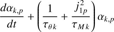
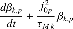
reasonable approximation to express Equations (14.162) and (14.163) in the simplified forms [16]
th rational surface. Hence, it is a
reasonable approximation to express Equations (14.162) and (14.163) in the simplified forms [16]
![$\displaystyle 4\pi^{2}\,R_0\left[\rho_k\,r^{3}\,\frac{\partial{\mit\Delta\Omega...
...r^{3}\,\frac{\partial{\mit\Delta\Omega}_{\theta\,k}}{\partial r}\right)
\right]$](img4451.png) |
 |
(14.166) |
![$\displaystyle 4\pi^{2}\,R_0^{\,3}\left[\rho_k\,r\,\frac{\partial{\mit\Delta\Ome...
...t(
r\,\frac{\partial{\mit\Delta\Omega}_{\varphi\,k}}{\partial r}\right) \right]$](img4452.png) |
 |
(14.167) |
 ,
,
 , and
, and
 .
where
Here,
.
where
Here,  is a Bessel function, and
  denotes its
  th zero [1]. Note that
Equations (14.168)–(14.171) automatically satisfy the boundary conditions (14.164) and (14.165).
th zero [1]. Note that
Equations (14.168)–(14.171) automatically satisfy the boundary conditions (14.164) and (14.165).
It is easily demonstrated that [33]
 |
 |
(14.172) |
 |
 |
(14.173) |
 |
![$\displaystyle = \frac{r_{100}^{4}}{2}\,[J_2(j_{1p})]^{\,2}\,\delta_{pq},$](img4465.png) |
(14.174) |
 |
![$\displaystyle = \frac{r_{100}^{2}}{2}\,[J_1(j_{0p})]^{\,2}\,\delta_{pq}.$](img4467.png) |
(14.175) |
Equations (14.69), (14.70), and (14.166)–(14.175) yield
Here, The values of ,
,
 ,
,
 , and
, and
 at the rational surfaces in our example
tokamak discharge are specified in Table 14.8.
Incidentally, Equations (14.176) and (14.177) are the toroidal generalizations of the cylindrical equations (3.190) and (3.191), respectively.
at the rational surfaces in our example
tokamak discharge are specified in Table 14.8.
Incidentally, Equations (14.176) and (14.177) are the toroidal generalizations of the cylindrical equations (3.190) and (3.191), respectively.
Let us define the frequency shifts that develop at the various rational surfaces in the plasma in response to the electromagnetic torques:
 |
(14.183) |
Consider an tearing mode that reconnects magnetic flux principally at the th rational surface in our example tokamak discharge.
Let
 be the normalized magnetic flux reconnected at the th surface, and let us suppose that
 is sufficiently large
that the plasma response at the th surface lies in the nonlinear regime. Because of the assumed strong shielding at the
other rational surfaces in the plasma, we expect the plasma responses at these surfaces to lie in the linear regime.
is sufficiently large
that the plasma response at the th surface lies in the nonlinear regime. Because of the assumed strong shielding at the
other rational surfaces in the plasma, we expect the plasma responses at these surfaces to lie in the linear regime.
We can determine the normalized reconnected magnetic fluxes,
 , driven at the other rational surfaces from Equations (14.119), (14.123),
(14.146), and (14.182).
We find that
, driven at the other rational surfaces from Equations (14.119), (14.123),
(14.146), and (14.182).
We find that
 |
(14.186) |
 . Hence,
for ,
where
. Hence,
for ,
where
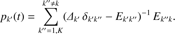
The normalized electromagnetic torque acting at the  th (where ) rational surface is
th rational surface is obtained from
angular momentum conservation (see Section 14.11):
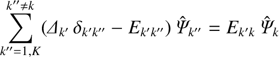
According to Equation (14.151), the frequency shift at the th rational surface modifies the real frequency of the
tearing mode. In fact,
![\includegraphics[width=\textwidth]{Chapter14/Figure14_4.eps}](img4514.png)
|
The normalized linear layer response indicies,
 (where ), that appear in Equation (14.188), are functions
of nine normalized layer parameters. (See Table 14.3.) Two of these parameters,
(where ), that appear in Equation (14.188), are functions
of nine normalized layer parameters. (See Table 14.3.) Two of these parameters,  and
and  , are modified
by the frequency shifts induced by the electromagnetic torques. In fact, it is clear from Equations (14.130), (14.131),
(14.185), and (14.191) that
, are modified
by the frequency shifts induced by the electromagnetic torques. In fact, it is clear from Equations (14.130), (14.131),
(14.185), and (14.191) that
 indicates a quantity that is unaffected by the electromagnetic torques.
Equations (14.176), (14.177), (14.184), (14.188)–(14.190), (14.192), (14.193)—together with the numerical solution of the Riccati differential
equation, (5.121), subject to the boundary conditions (5.122) and (5.123), which determines the
 —
form a closed set of equations that allow us to determine the reconnected magnetic fluxes driven at the various rational surfaces in our example tokamak
discharge by a tearing mode that reconnects magnetic flux primarily at the th rational surface. The only free parameter in the model
is the normalized reconnected magnetic flux at the th rational surface,
—
form a closed set of equations that allow us to determine the reconnected magnetic fluxes driven at the various rational surfaces in our example tokamak
discharge by a tearing mode that reconnects magnetic flux primarily at the th rational surface. The only free parameter in the model
is the normalized reconnected magnetic flux at the th rational surface,
 .
.
Consider an tearing mode in our example tokamak discharge that reconnects magnetic
flux principally at the  (i.e.,
  ) rational surface. Such a mode could represent an
  neoclassical
tearing mode. It is helpful to define the natural frequencies at the various rational surfaces in the plasma:
neoclassical
tearing mode. It is helpful to define the natural frequencies at the various rational surfaces in the plasma:
 |
 |
(14.194) |
 |
 |
(14.195) |
 , 3, 4, where
 and
and
 are specified in Table 14.5. Here, we are taking into account the fact that the plasma response at the rational surface lies
in the nonlinear regime (because the island width is assumed to be greater than the corresponding linear layer width),
whereas the plasma responses at the other rational surfaces lie in the linear regime (because the driven island
widths are assumed to be less than the corresponding linear layer widths). Moreover, we are also taking into account the
modifications to the natural frequencies generated by the electromagnetic torques that develop at the rational surfaces.
Recall that the natural frequency at a given rational surface is the preferred rotation frequency of reconnected
magnetic flux at that surface.
are specified in Table 14.5. Here, we are taking into account the fact that the plasma response at the rational surface lies
in the nonlinear regime (because the island width is assumed to be greater than the corresponding linear layer width),
whereas the plasma responses at the other rational surfaces lie in the linear regime (because the driven island
widths are assumed to be less than the corresponding linear layer widths). Moreover, we are also taking into account the
modifications to the natural frequencies generated by the electromagnetic torques that develop at the rational surfaces.
Recall that the natural frequency at a given rational surface is the preferred rotation frequency of reconnected
magnetic flux at that surface.
![\includegraphics[width=\textwidth]{Chapter14/Figure14_5.eps}](img4527.png)
|
Figure 14.4 shows the natural frequencies in our example tokamak
discharge calculated as functions of the normalized magnetic island width,
 ,
in a simulation in which the island width is slowly ramped up. This calculation is made using the
previously mentioned closed set of equations, as well as the data given in Tables 14.1, 14.2, 14.3, 14.5, and 14.8.
It can be seen that if
lies close to zero then the natural frequencies all take the unperturbed values specified in
Table 14.5. On the other hand, as
increases, the electromagnetic torques that develop at the rational
surfaces modify the natural frequencies. In particular, the torques cause the natural frequency,
,
in a simulation in which the island width is slowly ramped up. This calculation is made using the
previously mentioned closed set of equations, as well as the data given in Tables 14.1, 14.2, 14.3, 14.5, and 14.8.
It can be seen that if
lies close to zero then the natural frequencies all take the unperturbed values specified in
Table 14.5. On the other hand, as
increases, the electromagnetic torques that develop at the rational
surfaces modify the natural frequencies. In particular, the torques cause the natural frequency,
 , and the
 natural frequency,
 , to approach one another. At a critical value of
, which is approximately 0.41, the two natural
frequencies suddenly snap together, indicating a sudden loss of shielding at the rational surface [14].
, to approach one another. At a critical value of
, which is approximately 0.41, the two natural
frequencies suddenly snap together, indicating a sudden loss of shielding at the rational surface [14].
The aforementioned sudden loss of shielding
is illustrated in Figure 14.5, which shows the driven normalized magnetic island widths at the , 4, and 5 rational surfaces in our example
discharge as functions
of the normalized island width. It can be seen that, prior to the loss of shielding, comparatively narrow magnetic island chains are
driven at the , 4, and 5 rational surfaces. However, as soon as the shielding at the rational surface is lost, there is a
very significant increase in the width of the magnetic island chain driven at the surface.
![\includegraphics[width=\textwidth]{Chapter14/Figure14_6.eps}](img4533.png)
|
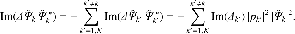
Finally, Figure 14.6 shows the normalized electromagnetic torques that develop at the rational surfaces in our example discharge close to the time at
which shielding is lost at the rational surface. It can be seen that the sudden loss of shielding is due to comparatively large transient
electromagnetic torques that develop at the and rational surfaces, and drive the corresponding natural frequencies together.
The calculation that we have just performed indicates that the shielding of rational surfaces from one another, as a consequence of
sheared rotation, in our example tokamak discharge is a very robust effect. In fact, the shielding only breaks down when a tearing mode
grows to a sufficient amplitude that the width of its magnetic island chain becomes a substantial fraction of the plasma minor radius. However,
when shielding breaks down, it does so in a sudden and catastrophic manner [14]. In fact, in our example calculation, the loss of
shielding at the rational surface drives a magnetic island chain at that surface whose width is sufficient that the chain
would overlap with the chain at the rational surface, leading to the sudden destruction of magnetic flux-surfaces [26], which could
quite conceivably trigger a disruption [7].

![$\displaystyle 4\pi^{2}\,R_0\left[\rho\,r^{\,3}\,\frac{\partial{\mit\Delta\Omega...
...r^{3}\,\frac{\partial{\mit\Delta\Omega}_{\theta\,k}}{\partial r}\right)
\right]$](img4441.png)
![$\displaystyle 4\pi^{2}\,R_0^{\,3}\left[\rho\,r\,\frac{\partial{\mit\Delta\Omega...
...}\,r\,\frac{\partial{\mit\Delta\Omega}_{\varphi\,k}}{\partial r}\right) \right]$](img4443.png)


![$\displaystyle = \frac{m_k^{2}\,[J_1(j_{1p}\,r_k/r_{100})]^{\,2}}{\tau_{A\,k}^{\...
..._{1p})]^{\,2}}\,
{\rm Im}({\mit\Delta\hat{\Psi}_k}\,\hat{\mit\Psi}_k^{\,\ast}),$](img4469.png)
![$\displaystyle = \frac{n^{2}\,[J_0(j_{0p}\,r_k/r_{100})]^{\,2}}{\tau_{A\,k}^{\,2...
..._{0p})]^{\,2}}\,
{\rm Im}({\mit\Delta\hat{\Psi}_k}\,\hat{\mit\Psi}_k^{\,\ast}).$](img4471.png)