Next: Linear Calculation Up: Toroidal Tearing Modes Previous: Toroidal Tearing Mode Dispersion Contents
![\includegraphics[width=1.\textwidth]{Chapter14/Figure14_2.eps}](img4219.png)
|
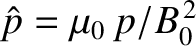
KSTAR discharge #18594 [29] is a typical H-mode [34] discharge in a mid-sized tokamak. Figure 14.1 shows the equilibrium
magnetic flux-surfaces in this discharge at time  ms, at which time
  T,
T,
 m,
m,
 m, and
 . Figures 14.2 and 14.3 show the corresponding pressure, safety-factor, and
  profiles [29]. Of course, the
equilibrium flux-surfaces shown in Figure 14.1, combined with the
profiles [29]. Of course, the
equilibrium flux-surfaces shown in Figure 14.1, combined with the  and profiles specified in Figures 14.2 and 14.3,
constitute a solution of the Grad-Shafranov equation, (14.33).
Note that the safety-factor
becomes infinite at the edge of the plasma, due to the presence of a magnetic X-point on the bounding magnetic flux-surface. (See Figure 14.1.)
In principle, there are an infinite number of
and profiles specified in Figures 14.2 and 14.3,
constitute a solution of the Grad-Shafranov equation, (14.33).
Note that the safety-factor
becomes infinite at the edge of the plasma, due to the presence of a magnetic X-point on the bounding magnetic flux-surface. (See Figure 14.1.)
In principle, there are an infinite number of  rational surfaces lying within the plasma. However, if we truncate the plasma at
 (i.e., at the magnetic flux-surface that contains 99.5% of the poloidal magnetic flux contained by the last closed flux-surface),
which is the standard approach, then there
are only four such surfaces. The properties of these surfaces are listed in Table 14.1.
(i.e., at the magnetic flux-surface that contains 99.5% of the poloidal magnetic flux contained by the last closed flux-surface),
which is the standard approach, then there
are only four such surfaces. The properties of these surfaces are listed in Table 14.1.
Table 14.2 specifies the elements of the E-matrix in KSTAR discharge #18594 at
time ms, calculate according to the procedure set out in Section 14.12. As expected, it can be seen that the matrix is Hermitian. Moreover, all of the diagonal
elements of the matrix are negative, which indicates that the tearing mode are all
classically stable. (This is not surprising because the classical drive is absent from our calculation.) Finally, the
off-diagonal elements of the matrix are all substantial, indicating that there is significant coupling between different poloidal harmonics.
In order to determine the effective tearing stability index for an toroidal tearing mode that reconnects magnetic flux at a particular
rational surface in the plasma, let us assume that the responses of the other rational surfaces exhibit strong shielding. This assumption can be justified a posteriori. Our assumption implies that very little
magnetic reconnection is driven at the other rational surfaces. In this case, it is reasonable to calculate the responses of these surfaces
using linear theory. (The linear approximation is valid as long as the widths of the magnetic island chains driven at the
other rational surfaces are less than the corresponding linear layer widths. See Section 5.16.)
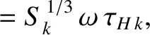
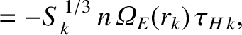
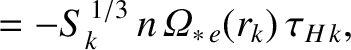
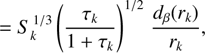
According to the analysis of Chapter 5, the linear response of the  th rational surface is
characterized by
th rational surface is
characterized by
 |
 |
(14.124) |
 |
 |
(14.125) |
 |
 |
(14.126) |
 |
 |
(14.127) |
 |
 |
(14.128) |
 |
 |
(14.129) |
 |
 |
(14.130) |
 |
 |
(14.131) |
 |
 |
(14.132) |
 |
 |
(14.133) |
 |
 |
(14.134) |
 |
 |
(14.135) |
 |
![$\displaystyle = \frac{\sqrt{(5/3)\,m_i\,[T_e+(n_i/n_e)\,T_i+(n_I/n_e)\,T_I]}}{e\,B_0\,g},$](img4292.png) |
(14.136) |
 |
 |
(14.137) |
 |
 |
(14.138) |
 |
 |
(14.139) |
 |
 |
(14.140) |
 is the Lundquist number,
 the resistive diffusion time [see Equation (5.49)], and
 the
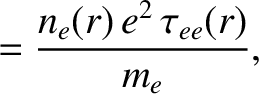
hydrodynamic time [see Equation (5.43)], at the th rational surface. Moreover,
the
hydrodynamic time [see Equation (5.43)], at the th rational surface. Moreover,  ,
,  ,
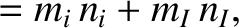
,  are the equilibrium number density profiles of the
electrons, majority ions, and impurity ions, respectively, whereas
are the equilibrium number density profiles of the
electrons, majority ions, and impurity ions, respectively, whereas  ,
,  , and
, and  are the corresponding temperature profiles, and
  ,
,  , and
, and  the corresponding
species masses. Furthermore,
the corresponding
species masses. Furthermore,  is the real frequency of the tearing mode in the laboratory frame, whereas the E-cross-B,
electron diamagnetic, and majority ion diamagnetic frequency profiles,
is the real frequency of the tearing mode in the laboratory frame, whereas the E-cross-B,
electron diamagnetic, and majority ion diamagnetic frequency profiles,
 ,
,
 , and
, and
 ,
respectively, are defined in Equations (A.77) and (A.78). The electron-electron collision time,
,
respectively, are defined in Equations (A.77) and (A.78). The electron-electron collision time,
 , is specified in Equation (A.23),
and
, is specified in Equation (A.23),
and  is the magnitude of the electron charge.
The dimensionless function
is the magnitude of the electron charge.
The dimensionless function
 , defined in Equation (A.81), specifies the reduction in the plasma electrical conductivity due to the presence of impurity
ions and trapped particles. (See Section 2.20.) In addition,
, defined in Equation (A.81), specifies the reduction in the plasma electrical conductivity due to the presence of impurity
ions and trapped particles. (See Section 2.20.) In addition,
 and
and
 are the toroidal momentum confinement time
[see Equation (5.50)] and the particle confinement time, respectively, at the th rational surface, whereas
are the toroidal momentum confinement time
[see Equation (5.50)] and the particle confinement time, respectively, at the th rational surface, whereas
 and
and
 are the ion perpendicular momentum diffusivity and perpendicular particle diffusivity profiles.
![\includegraphics[width=1.\textwidth]{Chapter14/Figure14_3.eps}](img4317.png)
|
Equation (14.123) states that the linear response of the th rational surface to a magnetic perturbation generated at another
rational surface is governed by nine dimensionless parameters. These parameters are the Lundquist number, , the normalized
mode frequency,  , the normalized E-cross-B frequency,
  , the normalized electron diamagnetic frequency,
  ,
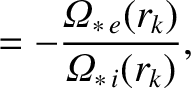
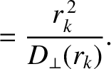
the normalized ion diamagnetic frequency,
,
the normalized ion diamagnetic frequency,  , the pressure gradient ratio parameter,
  , the semi-collisional
parameter,
, the semi-collisional
parameter,  , and the two magnetic Prandtl numbers,
 and
and
 . (Note that these parameters
are called
. (Note that these parameters
are called  ,
,  ,
,  ,
,  ,
,  ,
,  ,
,
 , and
, and  , respectively, in Chapter 5.) The dimensionless
layer response index,
, respectively, in Chapter 5.) The dimensionless
layer response index,
 , can be calculated numerically as a function of these nine parameters by solving the Riccati differential
equation, (5.121), subject to the boundary conditions (5.122) and (5.123).
, can be calculated numerically as a function of these nine parameters by solving the Riccati differential
equation, (5.121), subject to the boundary conditions (5.122) and (5.123).
Figure 14.3 shows the experimental number density, temperature, and E-cross-B frequency profiles in KSTAR discharge #18594 at
time ms [29].
The majority ions are deuterium, whereas the impurity ions are carbon-VI (i.e.,  ). The majority ion and impurity ion number density profiles are
calculated from the measured electron number density profile [see Equations (A.4) and (A.5)] on the assumption that the effective ion charge number,
). The majority ion and impurity ion number density profiles are
calculated from the measured electron number density profile [see Equations (A.4) and (A.5)] on the assumption that the effective ion charge number,
 [see Equation (A.3)],
takes the value
[see Equation (A.3)],
takes the value  throughout the plasma. (This value is a best guess based on the measured stored energy.) The impurity ions are assumed to have the same temperature as the measured temperature of the majority ions.
The E-cross-B frequency profile is deduced from the measured impurity ion toroidal angular velocity profile using the neoclassical
theory outlined in Appendix A [15]. In particular, the impurity ion poloidal angular velocity profile is assumed to take its neoclassical value. (See Section A.7). Furthermore, the
ion perpendicular momentum and perpendicular particle diffusivities are given the plausible values
throughout the plasma. (This value is a best guess based on the measured stored energy.) The impurity ions are assumed to have the same temperature as the measured temperature of the majority ions.
The E-cross-B frequency profile is deduced from the measured impurity ion toroidal angular velocity profile using the neoclassical
theory outlined in Appendix A [15]. In particular, the impurity ion poloidal angular velocity profile is assumed to take its neoclassical value. (See Section A.7). Furthermore, the
ion perpendicular momentum and perpendicular particle diffusivities are given the plausible values
 and
and
 , respectively, throughout the plasma [34]. Finally, the values of the various resistive layer parameters, determined from the data shown in Figure 14.3,
as well as the aforementioned assumptions, are given in Table 14.3.
, respectively, throughout the plasma [34]. Finally, the values of the various resistive layer parameters, determined from the data shown in Figure 14.3,
as well as the aforementioned assumptions, are given in Table 14.3.