Next: Bibliography Up: Linear Resonant Response Model Previous: Plasma Rotation Contents
 response regime. According to Equation (5.33),
the perturbed helical magnetic flux in the layer takes the form:
response regime. According to Equation (5.33),
the perturbed helical magnetic flux in the layer takes the form:
 |
(5.125) |
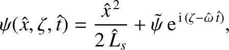
 is a complex constant. Of course, the physical flux is the real part of the previous expression; that is,
where
is a complex constant. Of course, the physical flux is the real part of the previous expression; that is,
where
 |
(5.127) |
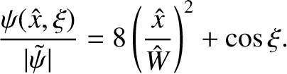
 . In other words, the contours of
 map out the perturbed magnetic flux-surfaces in the vicinity of the resonant layer.
Let
map out the perturbed magnetic flux-surfaces in the vicinity of the resonant layer.
Let
 . Equation (5.126) can be written
 |
(5.128) |
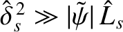
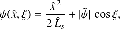
Figure 5.7 shows the contours of
specified by the previous equation. It can be seen that the tearing mode has changed the
topology of the magnetic field in the immediate vicinity of the rational surface,  . In fact, as the
tearing mode grows in amplitude (i.e., as
. In fact, as the
tearing mode grows in amplitude (i.e., as
 increases), magnetic field-lines pass through
the magnetic “X-points” (which are located at ,
increases), magnetic field-lines pass through
the magnetic “X-points” (which are located at ,
 , where
  is an integer), at which time they break (or “tear”) and then reconnect to form new field-lines that do not extend over all values of
  . The magnetic field-line
that forms the boundary between the unreconnected and reconnected regions is known as the magnetic
separatrix, and corresponds to the contour
. The magnetic field-line
that forms the boundary between the unreconnected and reconnected regions is known as the magnetic
separatrix, and corresponds to the contour
 . The reconnected regions within the
magnetic separatrix are termed magnetic islands.
The tearing mode clearly generates a chain of magnetic islands, centered on the rational surface, with
. The reconnected regions within the
magnetic separatrix are termed magnetic islands.
The tearing mode clearly generates a chain of magnetic islands, centered on the rational surface, with  periods in the poloidal direction, and
  periods in the toroidal direction, which propagates in the laboratory frame at the helical phase velocity
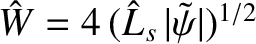
  . The maximum full (as opposed to half) radial width of the magnetic separatrix is
 is the reconnected magnetic flux defined in Equation (3.72), and
 .
.
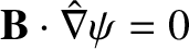
Finally, our reduced drift-MHD model, (5.10)–(5.13), contains many term of the general form
![$[\psi,\tilde{A}]$](img2346.png) ,
where
,
where
 is a perturbed quantity. According to Equation (5.126), such terms
can be written
is a perturbed quantity. According to Equation (5.126), such terms
can be written
![$\displaystyle [\psi,\tilde{A}] = {\rm i}\,\frac{m}{r_s}\left(\frac{\hat{x}}{\ha...
...de{A} - {\rm i}\,\frac{m}{r_s}\,\frac{\tilde{\psi}}{\hat{\delta}_s}\,\tilde{A},$](img2348.png) |
(5.130) |
 is the radial width of the linear layer. Now, linear layer theory is only valid when the second
term on the extreme right side of the previous equation is negligible compared to the first (because the second term is quadratic in perturbed quantities, whereas the first is linear). In other words,
we require
is the radial width of the linear layer. Now, linear layer theory is only valid when the second
term on the extreme right side of the previous equation is negligible compared to the first (because the second term is quadratic in perturbed quantities, whereas the first is linear). In other words,
we require
 , which reduces to
 |
(5.131) |
![\includegraphics[width=1.\textwidth]{Chapter05/Figure5_7.eps}](img2336.png)
