Next: Resonant Layer Equations Up: Linear Resonant Response Model Previous: Plasma Equilibrium Contents
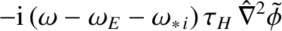
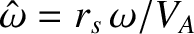 , and
, and  is the rotation frequency of the tearing perturbation in the laboratory frame.
Here,
is the rotation frequency of the tearing perturbation in the laboratory frame.
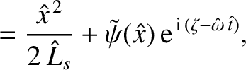
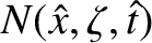
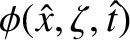
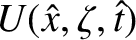
Here,  denotes a perturbed quantity.
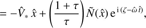
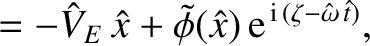
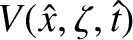
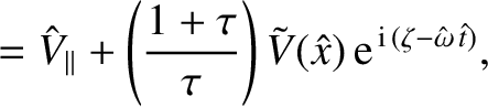
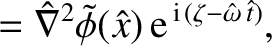
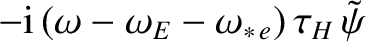
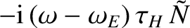
Substituting Equations (5.33)–(5.38) into the reduced drift-MHD model, (5.8)–(5.13), and only retaining terms that
are first order in perturbed quantities, we obtain the following set of linear equations:
Here,
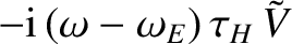
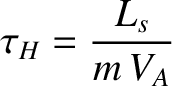
is the hydromagnetic time,
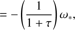
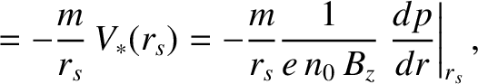
the
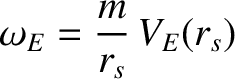
E-cross-B frequency,
the electron diamagnetic
frequency,
the ion diamagnetic
frequency,
the (total) diamagnetic frequency,
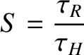
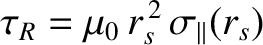
the Lundquist number [note that this is a slightly different definition to that given in Equation (1.84)],
the
resistive diffusion time [note that this is a slightly different definition to that given in Equation (1.83)],
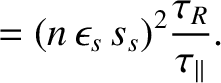
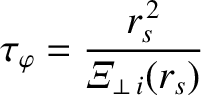
the toroidal momentum confinement time,
the effective parallel energy equilibration time, and
the effective energy confinement time.
Furthermore,
denotes a perturbed quantity.
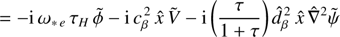
Substituting Equations (5.33)–(5.38) into the reduced drift-MHD model, (5.8)–(5.13), and only retaining terms that
are first order in perturbed quantities, we obtain the following set of linear equations:
Here,
is the hydromagnetic time,
the
E-cross-B frequency,
the electron diamagnetic
frequency,
the ion diamagnetic
frequency,
the (total) diamagnetic frequency,
the Lundquist number [note that this is a slightly different definition to that given in Equation (1.84)],
the
resistive diffusion time [note that this is a slightly different definition to that given in Equation (1.83)],
the toroidal momentum confinement time,
the effective parallel energy equilibration time, and
the effective energy confinement time.
Furthermore,
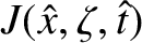

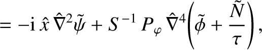


![$\displaystyle \tau_\parallel = r_s^{\,2}\left/\left\{\frac{2}{3}\,(1-c_\beta^2)...
...ft(\frac{\eta_i}{1+\eta_i}\right)\chi_{\parallel\,i}(r_s)\right]\right\}\right.$](img2062.png)
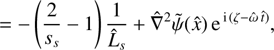
![$\displaystyle \tau_\perp =r_s^{\,2}\left/\left\{\frac{2}{3}\,(1-c_\beta^2)\left...
...)\left(\frac{\eta_i}{1+\eta_i}\right)\chi_{\perp\,i}(r_s)\right]\right\}\right.$](img2063.png)