Resonant Layer Equations

In a conventional tokamak plasma, the Lundquist number, $S$, which is the nominal ratio of the plasma inertia term to the resistive diffusion term in the plasma Ohm's law [14], is very much greater than unity. In fact, according to Table 1.5, $S$ typically exceeds $10^8$ in a tokamak fusion reactor. However, a resonant layer is characterized by a balance between plasma inertia and resistive diffusion [17]. Such a balance is only possible if the layer is very narrow in the radial direction (because a narrow layer enhances radial derivatives, and, thereby, enhances resistive diffusion). Let us define the stretched radial variable [2]

$$X = S^{1/3}\,\hat{x}.$$ (5.56)

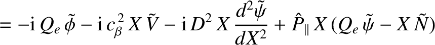
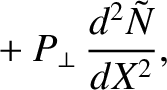
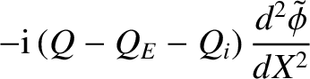
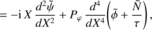
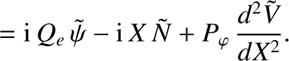
Assuming that $X\sim{\cal O}(1)$ in the layer (i.e., assuming that the layer thickness is roughly of order $S^{-1/3}\,r_s$), and making use of the fact that $S\gg 1$, we deduce that $\hat{\nabla}^2\simeq\hat{\nabla}_\perp^2\simeq S^{2/3}\,d^2/dX^2$. Hence, the linear equations (5.39)–(5.42) reduce to the following set of resonant layer equations [7,15]:

$$-{\rm i}\,(Q-Q_E-Q_{e})\,\tilde{\psi} = - {\rm i}\,X\,(\skew{3}\tilde{\phi}-\tilde{N})+ \frac{d^2\tilde{\psi}}{d X^2},$$ (5.57)

$$-{\rm i}\,(Q-Q_E)\,\tilde{N} = - {\rm i}\,Q_{e}\,\skew{3}\tilde{\phi} - {\rm i}\,c_\beta^{\,2}... ...2\tilde{\psi}}{dX^{2}}+\hat{P}_\parallel\,X\,(Q_e\,\tilde{\psi} - X\,\tilde{N})$$

$$\phantom{=} + P_\perp\,\frac{d^2 \tilde{N}}{dX^{2}},$$ (5.58)

$$-{\rm i}\,(Q-Q_E -Q_{i})\,\frac{d^2\skew{3}\tilde{\phi}}{dX^2} = - {\rm i}\,X\,\frac{d^2\tilde{\psi}}{dX^2}+ P_\varphi\,\frac{d^4}{dX^4}\!\left(\skew{3}\tilde{\phi} + \frac{\tilde{N}}{\tau}\right),$$ (5.59)

$$-{\rm i}\,(Q-Q_E)\,\tilde{V} = {\rm i}\,Q_{e}\,\tilde{\psi} - {\rm i}\,X\,\tilde{N} + P_\varphi\,\frac{d^2\tilde{V}}{dX^{2}}.$$ (5.60)

Here,

$$Q =S^{1/3}\,\omega\,\tau_H,$$ (5.61)

$$Q_E = S^{1/3}\,\omega_E\,\tau_H,$$ (5.62)

$$Q_{e} =S^{1/3}\,\omega_{\ast\,e}\,\tau_H= \left(\frac{\tau}{1+\tau}\right)Q_\ast,$$ (5.63)

$$Q_i =S^{1/3}\,\omega_{\ast\,i}\,\tau_H=- \left(\frac{1}{1+\tau}\right)Q_\ast,$$ (5.64)

$$Q_\ast = S^{1/3}\,\omega_\ast\,\tau_H,$$ (5.65)

$$D = S^{1/3}\left(\frac{\tau}{1+\tau}\right)^{1/2}\hat{d}_\beta,$$ (5.66)

$$\hat{P}_\parallel = \frac{P_\parallel}{S^{4/3}}.$$ (5.67)

Table: 5.1 Dimensionless parameters appearing in resonant layer equations for a low-field and a high-field tokamak reactor. See Equations (4.5), (5.65), (5.66), (5.53), (5.54), and (4.65).

	Low-Field	High-Field
$B({\rm T})$	5.0	12.0
$\tau$	1.0	1.0
$Q_\ast$	$2.00$	$1.50$
$D$	3.02	2.26
$P_\varphi$	874	874
$P_\perp$	287	287
$\hat{P}_\parallel$	0.635	0.635
$c_\beta$	0.128	0.128

Table 5.1 gives estimates for the values of the dimensionless parameters that characterize the resonant layer equations, (5.57)–(5.60), in a low-field and a high-field tokamak fusion reactor. (See Chapter 1.) These estimates are made using the following assumptions: $B=5\,{\rm T}$ (low-field) or $B=12\,{\rm T}$ (high-field), $\beta=0.02$, $T_e=T_i=7\,{\rm keV}$, $m_i=(m_D+m_T)/2$ (where $m_D$ and $m_T$ are the deuteron and triton masses, respectively), ${\mit\Xi}_{\perp\,i}= \chi_{\perp\,e}= \chi_{\perp\,i} = 1\,{\rm m^2/s}$, $m=2$, $n=1$, $r_s=a/2$ (where $a$ is the minor radius of the plasma), $s_s=1$, $\tau =1$, $\eta_e=\eta_i=1$, and $dp/dr=-p/a$. The parallel energy diffusivities, $\chi_{\parallel\,e}$ and $\chi_{\parallel\,e}$, are estimated from Equations (2.319) and (2.320), respectively, using $k_\parallel \simeq (m/L_s)\,S^{-1/3}$, which is the typical parallel wavenumber of the tearing perturbation at the edge of a resistive layer whose characteristic thickness is $S^{-1/3}\,r_s$. 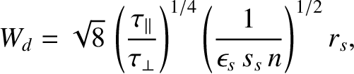Note that $\hat{P}_\parallel\ll P_\perp$, which allows us to neglect the parallel transport terms (i.e., the terms involving $\hat{P}_\parallel$) in Equation (5.58). The neglect of these terms is justified because the linear layer width is much less than the critical width,

$$W_d= \sqrt{8}\,\left(\frac{\tau_\parallel}{\tau_\perp}\right)^{1/4}\left(\frac{1}{\epsilon_s\,s_s\,n}\right)^{1/2}r_s,$$ (5.68)

below which parallel transport is unable to constrain the perturbed electron temperature to be constant along magnetic field-lines [12].