Next: Reduced Drift-MHD Model Up: Reduced Resonant Response Model Previous: Normalization Scheme Contents
 |
 |
(4.35) |
 |
 |
(4.36) |
 , only. Here,
  and
and  are the poloidal and toroidal mode numbers, respectively, of the tearing mode,
 is a simulated toroidal angle, and
  is the simulated major radius of the plasma. (See Chapter 3.)
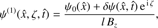
Let
where and
and
 . Here,
  is the safety factor profile. [See Equation (3.2).] Moreover, the superscript
  indicates a quantity that is
first order in our ordering scheme. [Zeroth order terms are left without superscripts, whereas second order terms are given the superscript (2).]
indicates a quantity that is
first order in our ordering scheme. [Zeroth order terms are left without superscripts, whereas second order terms are given the superscript (2).]
It follows that
for any . Furthermore,
 |
 |
(4.39) |
 |
 |
(4.40) |
 .
.
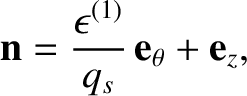
We can automatically satisfy Equation (4.32) by writing
It follows that where [see Equations (3.1) and (3.2)]![$\displaystyle \psi_0(\hat{x})=\frac{B_z}{R_0}\int_{r_s}^r r'\left[\frac{1}{q_s}-\frac{1}{q(r)}\right]dr',$](img1887.png) |
(4.43) |
 is defined in Equation (3.20).
Note that
is defined in Equation (3.20).
Note that
![$\displaystyle {\bf b}\cdot\hat{\nabla}A^{(1)} = \left[A^{(1)},\psi^{(1)}\right],$](img1888.png) |
(4.44) |
![$\displaystyle [A,B] \equiv \hat{\nabla} A\times \hat{\nabla} B\cdot{\bf n}.$](img1889.png) |
(4.45) |
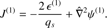
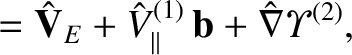
Equations (4.33) and (4.41) give
where |
(4.47) |
 which
generates the (normalized) inductive electric field,
which
generates the (normalized) inductive electric field,
 , that is responsible for maintaining the equilibrium parallel current density in the
inner region against ohmic decay.
, that is responsible for maintaining the equilibrium parallel current density in the
inner region against ohmic decay.
Equations (4.34) and (4.41) yield
 |
(4.48) |
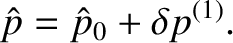
Let us write
Note that the ordering of the plasma pressure adopted here is somewhat different to that adopted in Section 3.3. In fact, in Section 3.3, was assumed to be second order. Here, we
are assuming that has a spatially constant component that is zeroth order, and a spatially
varying component that is first order. This high pressure ordering is merely an artifice to aid the
extraction of the compressible-Alfvén (i.e., fast magnetosonic) wave from the system of equations [3,4]. In fact, the ordering ensures that
the compressible-Alfvén wave has a substantially different phase velocity than the shear-Alfvén and slow magnetosonic waves [2].
was assumed to be second order. Here, we
are assuming that has a spatially constant component that is zeroth order, and a spatially
varying component that is first order. This high pressure ordering is merely an artifice to aid the
extraction of the compressible-Alfvén (i.e., fast magnetosonic) wave from the system of equations [3,4]. In fact, the ordering ensures that
the compressible-Alfvén wave has a substantially different phase velocity than the shear-Alfvén and slow magnetosonic waves [2].
Equations (4.28)–(4.31), (4.41), (4.46), and (4.50) yield
Here, the additional factor involving in Equation (4.53) is needed because
the plasma flow is slightly compressible. In fact, the velocity fields
in Equation (4.53) is needed because
the plasma flow is slightly compressible. In fact, the velocity fields
 ,
,
 ,
,
 , and
, and
 all have normalized divergences
that are second order.
all have normalized divergences
that are second order.
Evaluating the normalized drift-MHD fluid equations, (4.25)–(4.27), up to second order, we obtain
To first order, Equations (4.55) and (4.56) both yield
which is simply an expression of lowest-order equilibrium force balance [3,7].
Taking the
scalar product of Equation (4.55) with  annihilates the first-order terms, leaving
annihilates the first-order terms, leaving
Furthermore, taking the scalar product of the curl of Equation (4.55) with annihilates the first-order terms,
leaving
where
Finally, taking the scalar product of the curl of Equation (4.56) with annihilates the first-order terms,
leaving
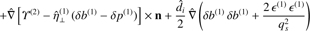
![$\displaystyle \hat{\nabla}^2{\mit\Upsilon}^{(2)} = 2\left[\delta p^{(1)}, \phi^{(1)}\right] +\hat{d}_i\left[J^{(1)}, \psi^{(1)}\right].$](img1924.png) |
(4.63) |

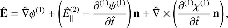


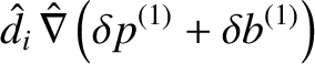
![$\displaystyle \hat{\nabla}\left(\delta p^{(1)}+ \delta b^{(1)}\right)+\left(\fr...
...l^{(1)},\phi^{(1)}\right] +\left[\psi^{(1)},\delta b^{(1)}\right]\right){\bf n}$](img1907.png)


![$\displaystyle +\left(\hat{E}_\parallel^{(2)}-\frac{\partial^{(1)}\psi^{(1)}}{\p...
...i^{(1)},\delta b^{(1)}\right]+\hat{\eta}_\parallel^{(1)}\,J^{(1)}\right){\bf n}$](img1911.png)

![$\displaystyle \frac{3}{2}\,\frac{\partial^{(1)}\delta p^{(1)}}{\partial\hat{t}}...
...{V}_\parallel^{(1)},\psi^{(1)}\right]+\hat{\nabla}^2{\mit\Upsilon}^{(2)}\right)$](img1914.png)
![$\displaystyle +\frac{5}{2}\,\lambda\,\hat{p}_0\,\hat{d}_i\,[\delta p^{(1)},\del...
...ight],\psi^{(1)}\right]-\hat{\chi}_\perp^{(1)}\,\hat{\nabla}^2\delta p^{(1)}=0.$](img1915.png)
![$\displaystyle \frac{\partial^{(1)}\hat{V}_\parallel^{(1)}}{\partial\hat{t}}=\le...
...{(1)}\right] +\hat{\mit\Xi}_\perp^{(1)}\,\hat{\nabla}^2\hat{V}_\parallel^{(1)}.$](img1918.png)
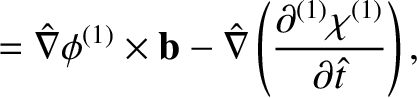
![$\displaystyle \frac{\partial^{(1)}\psi^{(1)}}{\partial \hat{t}}= \left[\phi^{(1...
...i^{(1)}\right] + \hat{\eta}_\parallel^{(1)}\,J^{(1)} + \hat{E}_\parallel^{(2)}.$](img1919.png)
![$\displaystyle = \left[\phi^{(1)},U^{(1)}\right]+\frac{\hat{d}_i}{2\,(1+\tau)}
\...
...ta p ^{(1)}\right]
+\left[\hat{\nabla}^2\delta p^{(1)},\phi^{(1)}\right]\right)$](img1921.png)
![$\displaystyle \phantom{=} +\left[J^{(1)},\psi^{(1)}\right] + \hat{\mit\Xi}_\per...
...hat{\nabla}^4\left(
\phi^{(1)}-\frac{\hat{d}_i}{1+\tau}\,\delta p^{(1)}\right),$](img1922.png)
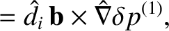
![$\displaystyle = \left[\phi^{(1)},\delta p^{(1)}\right]
-c_\beta^{\,2}\left[\hat...
...(1)},\psi^{(1)}\right] -c_\beta^{\,2}\,\hat{d}_i\left[J^{(1)},\psi^{(1)}\right]$](img1926.png)