Next: Normalization Scheme Up: Reduced Resonant Response Model Previous: Introduction Contents
 ,
,  ,
,  be conventional right-handed cylindrical coordinates, and let the rational magnetic flux-surface lie at
  .
It is helpful to define
the following parameters:
where
.
It is helpful to define
the following parameters:
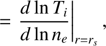
where  ,
,
 ,
,  , and
, and  refer to electron number density, total pressure, electron temperature, and ion temperature profiles, respectively, that are unperturbed by the tearing mode.
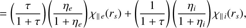
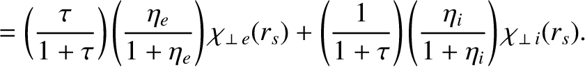
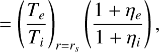
As has already been suggested, it is convenient to make the simplifying approximation that the perturbed electron and ion temperature profiles in the vicinity of the resonant
layer are functions of the perturbed electron number density profile. In other words,
 and
and
 .
It follows that the perturbed total pressure profile is also a function of the perturbed electron number density profile: that is,
.
It follows that the perturbed total pressure profile is also a function of the perturbed electron number density profile: that is,
 .
.
When stripped of specifically neoclassical terms (i.e., the ion poloidal flow damping terms, and any other terms
involving the superscript  ), our neoclassical fluid equations, (2.370)–(2.374), reduce to the following set of
drift-MHD fluid equations:
), our neoclassical fluid equations, (2.370)–(2.374), reduce to the following set of
drift-MHD fluid equations:
 is the magnetic field-strength,
  the electric field-strength,
  the current density,
 the ion fluid velocity,
  the ion mass,
 the
classical (see Section 2.6) perpendicular (to the equilibrium magnetic field) electrical conductivity,
the
classical (see Section 2.6) perpendicular (to the equilibrium magnetic field) electrical conductivity,
 the classical parallel electrical conductivity,
 the ion perpendicular momentum diffusivity,
 the
electron parallel energy diffusivity,
the
electron parallel energy diffusivity,
 the
ion parallel energy diffusivity,
the
ion parallel energy diffusivity,
 the
electron perpendicular energy diffusivity,
the
electron perpendicular energy diffusivity,
 the
ion perpendicular energy diffusivity, and
the
ion perpendicular energy diffusivity, and
 .
Note that the simplifying assumption that negates the need for a separate electron number density conservation equation. [In other words, Equation (2.370) is redundant.]
Moreover, Equation (4.9) is the sum of the electron and ion energy conservation equations, (2.373) and
(2.374).
In writing Equations (4.7)–(4.9), we have made a number of additional simplifying assumptions. For instance,
we have replaced
.
Note that the simplifying assumption that negates the need for a separate electron number density conservation equation. [In other words, Equation (2.370) is redundant.]
Moreover, Equation (4.9) is the sum of the electron and ion energy conservation equations, (2.373) and
(2.374).
In writing Equations (4.7)–(4.9), we have made a number of additional simplifying assumptions. For instance,
we have replaced  by
by  , which approximated as a spatial constant (see Section 3.3),
  by
by  (when a spatial or temporal derivative of the electron number density is not being taken), and
 by
by  (in the same circumstances). Finally, we have neglected any spatial
variation in transport coefficients (e.g.,
,
(in the same circumstances). Finally, we have neglected any spatial
variation in transport coefficients (e.g.,
,
 ,
) across the inner region.
,
) across the inner region.
Our drift-MHD fluid equations are closed by the following subset of Maxwell's equations:


![$\displaystyle m_i\,n_0\left[\frac{\partial {\bf V}}{\partial t} + ({\bf V}\cdot...
...au}\,({\bf V}_\ast\cdot\nabla){\bf V}_E\right]+\nabla p - {\bf j}\times {\bf B}$](img1803.png)