Next: Discussion Up: Plasma Fluid Theory Previous: Derivation of Neoclassical Fluid Contents
 |
 |
(2.354) |
 |
 |
(2.355) |
 |
 |
(2.356) |
 |
 |
(2.357) |
 |
 |
(2.358) |
 |
 |
(2.359) |
 |
 |
(2.360) |
 |
 |
(2.361) |
 is the typical time required for a sound wave to traverse the plasma,
 is the typical time required for electron energy to diffuse out of the plasma,
 is the typical time required for ion energy to diffuse out of the plasma,
 is the typical time required for momentum to diffuse out of the plasma,
 is the typical time required for the perpendicular current to diffuse out of the plasma,
 is the typical time required for the parallel current to diffuse out of the plasma,
 is the typical time required for the electron temperature to attain equilibrium on magnetic
flux-surfaces, and
is the typical time required for the electron temperature to attain equilibrium on magnetic
flux-surfaces, and
 is the typical time required for the ion temperature to attain equilibrium on magnetic
flux-surfaces. We shall assume that
is the typical time required for the ion temperature to attain equilibrium on magnetic
flux-surfaces. We shall assume that
 . We shall also assume that
The previous equation is an extension of the drift ordering, (2.113), that takes into
account the fact that tearing modes usually propagate with respect to the MHD fluid at diamagnetic velocities [2].
. We shall also assume that
The previous equation is an extension of the drift ordering, (2.113), that takes into
account the fact that tearing modes usually propagate with respect to the MHD fluid at diamagnetic velocities [2].
It is helpful to define the following dimensionless parameters:
Here, is the ion magnetization parameter defined in Equation (2.110), whereas
  is defined in Equation (1.23). Table 2.6 gives estimates for the
dimensionless parameters defined in Equations (2.363)–(2.369) for a low-field and a high-field fusion reactor. As before, these estimates are made
assuming that
is defined in Equation (1.23). Table 2.6 gives estimates for the
dimensionless parameters defined in Equations (2.363)–(2.369) for a low-field and a high-field fusion reactor. As before, these estimates are made
assuming that
 ,
,
 , and
, and  .
.
Our neoclassical fluid equations, (2.326), (2.331), and (2.338)–(2.340), can be written
Here, the factors![$[{\mit\Delta}_i]$](img1400.png) ,
,
![$[{\mit\Delta}_\theta]$](img1401.png) ,
,
![$[{\mit\Delta}_\perp]$](img1402.png) , et cetera, indicate that the terms they precede are larger or
smaller than terms preceded by no factor by the dimensionless parameter contained within the square brackets.
, et cetera, indicate that the terms they precede are larger or
smaller than terms preceded by no factor by the dimensionless parameter contained within the square brackets.
According to Table 2.6, the dominant parallel diffusivity term in the electron energy conservation equation, (2.373), yields
In other words, the parallel electron energy diffusivity in a tokamak fusion reactor is sufficiently large to ensure that the electron temperature is uniform on magnetic flux-surfaces. Likewise, according to Table 2.6, the dominant parallel diffusivity term in the ion energy conservation equation, (2.374), gives In other words, the parallel ion energy diffusivity in a tokamak fusion reactor is sufficiently large to ensure that the ion temperature is uniform on magnetic flux-surfaces. According to Table 2.6, the dominant terms in the plasma equation of motion, (2.371), yield In other words, the plasma in a tokamak fusion reactor exists in a state of approximate force balance. The previous equation suggests that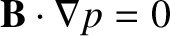 . When combined with Equations (2.375) and
(2.376), this relation gives
We conclude that the electron number density, the electron pressure, and the ion pressure are all
uniform on magnetic flux-surfaces in a tokamak fusion reactor. According to Table 2.6, the dominant terms in the plasma Ohm's law, (2.372), yield
where use has been made of Equations (2.377) and (2.378). Thus, we conclude that the
plasma in a tokamak fusion reactor satisfies the so-called perfect conductivity or flux-freezing constraint.
As is well known, this constraint forbids any change in the topology of magnetic field-lines [18].
Finally, according to Table 2.6, the dominant term in the electron number density continuity equation, (2.370), gives
Equations (2.375)–(2.380) are known collectively as the equations of marginally-stable ideal-MHD [20].
. When combined with Equations (2.375) and
(2.376), this relation gives
We conclude that the electron number density, the electron pressure, and the ion pressure are all
uniform on magnetic flux-surfaces in a tokamak fusion reactor. According to Table 2.6, the dominant terms in the plasma Ohm's law, (2.372), yield
where use has been made of Equations (2.377) and (2.378). Thus, we conclude that the
plasma in a tokamak fusion reactor satisfies the so-called perfect conductivity or flux-freezing constraint.
As is well known, this constraint forbids any change in the topology of magnetic field-lines [18].
Finally, according to Table 2.6, the dominant term in the electron number density continuity equation, (2.370), gives
Equations (2.375)–(2.380) are known collectively as the equations of marginally-stable ideal-MHD [20].


![$\displaystyle \frac{\partial n_e}{\partial t} + \nabla\cdot\left[n_e\,({\bf V} + {\bf V}_{\ast\,i})\right]=0,$](img1391.png)
![$\displaystyle m_i\,n_e\,\frac{\partial {\bf V}}{\partial t} + m_i\,n_e\left[({\...
...a){\bf V}_E\right]
+[{\mit\Delta}_i]\left(\nabla p -{\bf j}\times{\bf B}\right)$](img1392.png)
![$\displaystyle +[{\mit\Delta}_\theta]\,\frac{m_i\,n_e}{\tau_{\theta\,i}}\left(V_...
...\mit\Delta}_\perp]\,
\nabla\cdot(m_i\,n_e\,{\mit\Xi}_{\perp\,i}\,{\bf W}_i)= 0,$](img1393.png)
![$\displaystyle {\bf E}+ {\bf V}\times {\bf B} + \frac{1}{e\,n_e}\left(\nabla p -...
...p}]\,\eta_\perp^{nc}\left({\bf j}_\perp -\frac{{\bf b}\times\nabla p}{B}\right)$](img1394.png)
![$\displaystyle +[{\mit\Delta}_{R\,\parallel}]\, \eta_{\parallel}^{nc}\,(j_\parallel - j_\parallel^{\,nc})\,{\bf b},$](img1395.png)

![$\displaystyle -[{\mit\Delta}_{\parallel\,e}]\,\nabla\cdot(n_e\,\chi_{\parallel\...
...
-[{\mit\Delta}_\perp]\,\nabla\cdot(n_e\,\chi_{\perp\,e}\,\nabla_\perp\,T_e)=0,$](img1397.png)

![$\displaystyle -[{\mit\Delta}_{\parallel\,i}]\nabla\cdot(n_e\,\chi_{\parallel\,i...
...)
-[{\mit\Delta}_\perp]\nabla \cdot(n_e\,\chi_{\perp\,i}\,\nabla_\perp\,T_i)=0.$](img1399.png)

![$\displaystyle \frac{\partial n_e}{\partial t} + \nabla\cdot\left[n_e\,({\bf V} + {\bf V}_{\ast\,i})\right]\simeq 0.$](img1409.png)