Next: Normalization of Neoclassical Fluid Up: Plasma Fluid Theory Previous: Parallel Closure Scheme Contents
The electron and ion continuity equations, (2.26) and (2.29), can be combined with Equations (2.322), (2.323), and (2.325) to give an electron number density continuity equation of the form [29]:
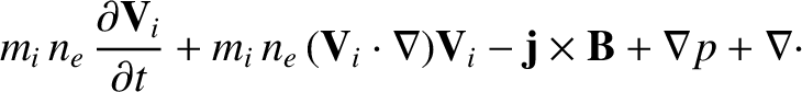
If we sum the electron and the ion equations of motion, (2.27) and (2.30), then we obtain
     |
(2.327) |
 is the total plasma pressure, and use has been made of Equations (2.16), (2.39), and (2.59). In the previous equation, we have neglected electron inertia with respect to ion inertia, because the former is
 times smaller than the latter. We have also neglected electron viscosity with respect to ion viscosity, because the former is, at least,
![${\cal O}[(m_e/m_i)^{1/2}]$](img1174.png) times smaller than the latter. Now, it can be demonstrated that [28,29]:
This important result is known as the gyro-viscous cancellation. Furthermore, it is clear from Equations (2.152)
and (2.161) that
times smaller than the latter. Now, it can be demonstrated that [28,29]:
This important result is known as the gyro-viscous cancellation. Furthermore, it is clear from Equations (2.152)
and (2.161) that


 acts predominately in the
 direction (i.e.,
parallel to
direction (i.e.,
parallel to
 ). A model form for
that is consistent with the analysis of
Section 2.18 is
where
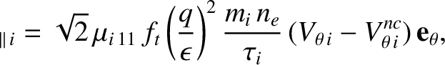
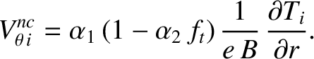
Thus, the neoclassical ion parallel viscosity tensor acts to relax the ion poloidal velocity toward the neoclassical
velocity specified in Equation (2.330) on a timescale that is roughly
). A model form for
that is consistent with the analysis of
Section 2.18 is
where
Thus, the neoclassical ion parallel viscosity tensor acts to relax the ion poloidal velocity toward the neoclassical
velocity specified in Equation (2.330) on a timescale that is roughly
 .
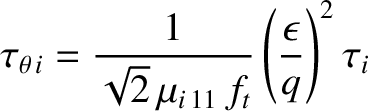
As has already been mentioned, this effect is known as poloidal flow damping. Equations (2.328) and (2.329)
can be combined with Equation (2.303) to give an MHD equation of motion of the form:
where
is the poloidal flow-damping time. Of course, the value of the anomalous perpendicular momentum
diffusivity,
.
As has already been mentioned, this effect is known as poloidal flow damping. Equations (2.328) and (2.329)
can be combined with Equation (2.303) to give an MHD equation of motion of the form:
where
is the poloidal flow-damping time. Of course, the value of the anomalous perpendicular momentum
diffusivity,
 , must be taken from experiments.
The electron equation of motion, (2.27), can be combined with Equations (2.59), (2.139) and (2.323) to give
Here, we have neglected electron inertia and gyro-viscosity, because these terms are times
smaller than the leading-order terms. We have also neglected anomalous electron perpendicular viscosity because there are no available experimental measurements of this effect in tokamak plasmas. Let us adopt the following
model form for
times
smaller than the leading-order terms. We have also neglected anomalous electron perpendicular viscosity because there are no available experimental measurements of this effect in tokamak plasmas. Let us adopt the following
model form for
 which is consistent with the analysis of Sections 2.16, 2.19, and 2.20:
where
which is consistent with the analysis of Sections 2.16, 2.19, and 2.20:
where
 |
 |
(2.335) |
 |
 |
(2.336) |
 |
 |
(2.337) |
 smaller than the similar term in the
previous equation that involves
smaller than the similar term in the
previous equation that involves
 .
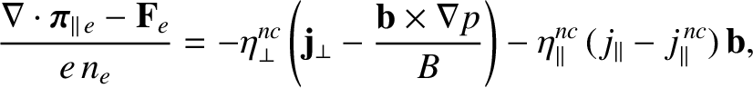
Thus, Equations (2.333) and (2.334) yield the following generalized Ohm's law for the plasma:
.
Thus, Equations (2.333) and (2.334) yield the following generalized Ohm's law for the plasma:
The electron and ion energy conservation equations, (2.28) and (2.31), yield the following electron and ion energy conservation equations:
 |
||
 |
(2.339) | |
 |
||
 |
(2.340) |
 |
 |
(2.341) |
 |
 |
(2.342) |
 |
 |
(2.343) |
 |
 |
(2.344) |
 ), because this is a small effect, due to the smallness of the mass ratio
  . [See Equation (2.37).] We have also
neglected ohmic heating (i.e.,
. [See Equation (2.37).] We have also
neglected ohmic heating (i.e.,
 ), because this effect is
![${\cal O}[(\rho_e/l_e)/\beta^{\,2}]\sim 10^{-4}$](img1323.png) (see Tables 1.2 and 2.1) smaller than the leading order terms. In addition, we have neglected viscous heating, because this effect is, at least,
(see Tables 1.2 and 2.1) smaller than the leading order terms. In addition, we have neglected viscous heating, because this effect is, at least,
 times smaller than the leading-order terms.
In accordance with the discussion in Section 2.23, we have neglected the parallel component of the thermal
heat flux, (2.47). We have also neglected the perpendicular component of the thermal heat flux because this term is
the same size as the classical electron perpendicular heat flux (and, therefore, much smaller than the anomalous
electron perpendicular heat flux). The parallel heat “diffusivities”,
times smaller than the leading-order terms.
In accordance with the discussion in Section 2.23, we have neglected the parallel component of the thermal
heat flux, (2.47). We have also neglected the perpendicular component of the thermal heat flux because this term is
the same size as the classical electron perpendicular heat flux (and, therefore, much smaller than the anomalous
electron perpendicular heat flux). The parallel heat “diffusivities”,
 and
and
 , are
given the collisionless values specified in Equations (2.319) and (2.320), respectively. Of course, the values of the anomalous perpendicular heat
diffusivities,
, are
given the collisionless values specified in Equations (2.319) and (2.320), respectively. Of course, the values of the anomalous perpendicular heat
diffusivities,
 and
and
 , must be taken from experiments.
Note, finally, that when combined with the following subset of Maxwell's equations,
our final set of neoclassical fluid equations, (2.326), (2.331), and (2.338)–(2.340), form a complete set.


![$\displaystyle \frac{\partial n_e}{\partial t} + \nabla\cdot\left[n_e\,({\bf V} + {\bf V}_{\ast\,i})\right]=0.$](img1270.png)
![$\displaystyle _{\times\,i}=
m_i\,n_e\left[\frac{\partial {\bf V}}{\partial t} + ({\bf V}\cdot\nabla){\bf V} + ({\bf V}_{\ast\,i}\cdot\nabla){\bf V}_E\right].$](img1278.png)