Next: Trapped and Passing Particles Up: Plasma Fluid Theory Previous: Fluid Closure Schemes Contents
 |
 |
(2.32) |
 |
 |
(2.33) |
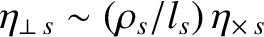
For particle, momentum, and energy flows perpendicular to magnetic field-lines, the small (compared to unity) dimensionless expansion parameters upon which the classical asymptotic closure scheme
is based are  and
and  . Here, we are assuming that the variation length-scales of quantities perpendicular to magnetic field-lines are
of order the plasma minor radius,
. Here, we are assuming that the variation length-scales of quantities perpendicular to magnetic field-lines are
of order the plasma minor radius,  . As is apparent from Table 2.2, the expansion parameters and are indeed small compared to unity in tokamak fusion reactors.
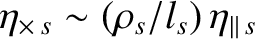
For particle, momentum, and energy flows parallel to magnetic field-lines, the small (compared to unity) expansion parameters upon which the classical asymptotic closure scheme
is based are  and
and  . Here, we are assuming that the variation length-scales of quantities parallel to magnetic field-lines are
of order the connection length,
. Here, we are assuming that the variation length-scales of quantities parallel to magnetic field-lines are
of order the connection length,
 , which is the typical distance a magnetic field-line has to travel in order to fully traverse a magnetic-flux surface. As is clear from Table 2.2, the expansion parameters and are actually both large compared to unity in tokamak fusion reactors. It follows that the classical asymptotic closure scheme fails in such reactors (because the confined plasmas are not sufficiently collisional in nature). Nevertheless, in the following, we shall describe the classical asymptotic closure scheme, before attempting to repair it.
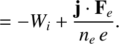
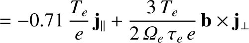
According to the classical asymptotic closure scheme [6],
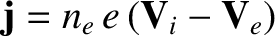
Here, is a unit vector parallel to the magnetic field, and
is the plasma current density.
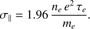
Moreover, the parallel electrical conductivity is given by [6,47]
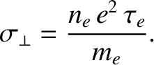
whereas the perpendicular electrical conductivity takes the form [6]
Note that
is a unit vector parallel to the magnetic field, and
is the plasma current density.
Moreover, the parallel electrical conductivity is given by [6,47]
whereas the perpendicular electrical conductivity takes the form [6]
Note that
![$\nabla_\parallel(\cdots) \equiv [{\bf b}\cdot\nabla
(\cdots)]\,{\bf b}$](img571.png) denotes a
gradient parallel to the magnetic field, whereas
denotes a
gradient parallel to the magnetic field, whereas
 denotes a gradient perpendicular to the magnetic
field. Likewise,
denotes a gradient perpendicular to the magnetic
field. Likewise,
 represents the component of the plasma current density flowing parallel to the
magnetic field, whereas
represents the component of the plasma current density flowing parallel to the
magnetic field, whereas
 represents the perpendicular component of the plasma current density.
It can be seen that parallel component of the friction force density,  , is smaller than the perpendicular component by a factor
  ; this is a consequence of the fact that the collision
frequency decreases with increasing velocity (
; this is a consequence of the fact that the collision
frequency decreases with increasing velocity (
 ), causing the distribution of electrons with large parallel velocities to be more distorted from a Maxwellian
distribution than that of slower electrons [30]. The thermal force density,
), causing the distribution of electrons with large parallel velocities to be more distorted from a Maxwellian
distribution than that of slower electrons [30]. The thermal force density,  , is also a consequence of the velocity dependence of the collision frequency [18]. (See Section 2.23.)
The electron and ion heat fluxes are written [6]
respectively, where are known as the parallel, cross, perpendicular, and thermal heat fluxes, respectively. Here, the parallel thermal conductivities, which control the diffusion of heat parallel to magnetic field-lines, are given by [6] Moreover, the cross thermal conductivities, which control the (non-diffusive) flow of heat within magnetic flux-surfaces, perpendicular to magnetic field-lines, are written [6] (See Section 2.11.) Finally, the perpendicular thermal conductivities, which control the diffusion of heat perpendicular to magnetic flux-surfaces, take the forms [6] Note that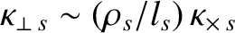 and
and
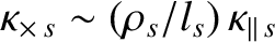 . In other words,
in a highly magnetized plasma (i.e.,
. In other words,
in a highly magnetized plasma (i.e.,
 ), the species-
 perpendicular thermal conductivity is much less than the cross conductivity, which,
in turn, is much less than the parallel conductivity.
perpendicular thermal conductivity is much less than the cross conductivity, which,
in turn, is much less than the parallel conductivity.
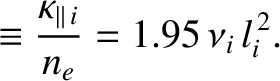
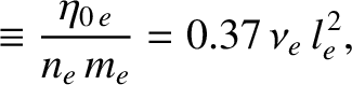
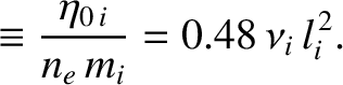
According to the previous expressions, the diffusion of heat parallel to magnetic field-lines is characterized by the diffusivities
 |
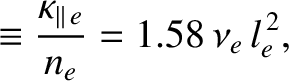 |
(2.54) |
 |
 |
(2.55) |
 and a step-length of order
  [18,41].
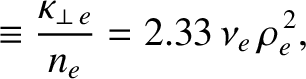
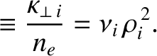
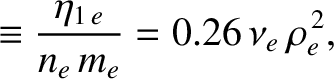
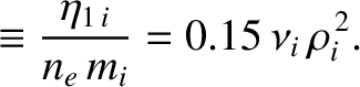
On the other hand, the diffusion of heat perpendicular to magnetic field-lines is characterized by the diffusivities
[18,41].
On the other hand, the diffusion of heat perpendicular to magnetic field-lines is characterized by the diffusivities
 |
 |
(2.56) |
 |
 |
(2.57) |
and a step-length of order
 [18,41].
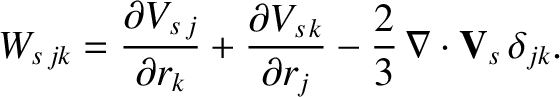
In order to describe the viscosity tensor in a highly magnetized plasma, it is
helpful to define the species- rate-of-strain tensor:
 |
(2.58) |
fluid
translates, or rotates as a rigid body, or if it undergoes isotropic
compression. Thus, the rate-of-strain tensor measures the deformation of
species- fluid volume elements.
In a highly magnetized plasma, the viscosity tensor is conveniently described as the sum of three component tensors [6]:
where  |
 |
(2.60) |
 |
 |
(2.61) |
 |
 |
(2.62) |
 is the identity tensor, and
 .
.
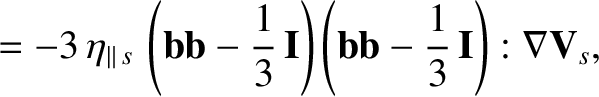
The tensor

 describes what is known as parallel viscosity; this is a viscosity that controls the diffusion of parallel (to the magnetic field) momentum along magnetic field-lines.
The parallel
viscosity coefficients are given by [6]
describes what is known as parallel viscosity; this is a viscosity that controls the diffusion of parallel (to the magnetic field) momentum along magnetic field-lines.
The parallel
viscosity coefficients are given by [6]
 |
 |
(2.63) |
 |
 |
(2.64) |
 describes what is known
as gyro-viscosity; this is not really viscosity at all, because the
associated viscous stresses are always perpendicular to the velocity, implying that
there is no dissipation (i.e., viscous heating) associated with
this effect. The gyro-viscosity coefficients are given by [6]
describes what is known
as gyro-viscosity; this is not really viscosity at all, because the
associated viscous stresses are always perpendicular to the velocity, implying that
there is no dissipation (i.e., viscous heating) associated with
this effect. The gyro-viscosity coefficients are given by [6]
 |
 |
(2.65) |
 |
 |
(2.66) |
 describes what is known
as perpendicular viscosity; this is a viscosity
that controls the diffusion of perpendicular momentum perpendicular to magnetic field-lines. The perpendicular
viscosity coefficients take the forms [6]
describes what is known
as perpendicular viscosity; this is a viscosity
that controls the diffusion of perpendicular momentum perpendicular to magnetic field-lines. The perpendicular
viscosity coefficients take the forms [6]
 |
 |
(2.67) |
 |
 |
(2.68) |
 and
and
 . In other words,
in a highly magnetized plasma (i.e.,
), the species- perpendicular viscosity is much less than the gyroviscosity, which,
in turn, is much less than the parallel viscosity.
. In other words,
in a highly magnetized plasma (i.e.,
), the species- perpendicular viscosity is much less than the gyroviscosity, which,
in turn, is much less than the parallel viscosity.
According to the previous expressions, the diffusion of parallel momentum parallel to magnetic field-lines is characterized by the diffusivities
 |
 |
(2.69) |
 |
 |
(2.70) |
and a step-length of order [18,41].
On the other hand, the diffusion of perpendicular momentum perpendicular to magnetic field-lines is characterized by the diffusivities
 |
 |
(2.71) |
 |
 |
(2.72) |
and a step-length of order
[18,41].
Table 2.3 shows estimates for the classical heat and momentum diffusivities in a tokamak
fusion reactor. It can be seen that the electron parallel diffusivities are much larger than the ion parallel diffusivities, but that both are extremely large. On the other hand, the ion perpendicular diffusivities are much larger than the electron perpendicular diffusivities, but both are
much smaller than the experimentally observed perpendicular diffusivities, which are all approximately
 [52].
[52].