Next: Neoclassical Closure Scheme Up: Plasma Fluid Theory Previous: Classical Closure Scheme Contents
 is the particle's perpendicular (to the magnetic field) velocity, and
  the local magnetic field-strength. Now, it is clear from Table 2.1
that the gyro-radii of both electrons and ions in a tokamak fusion reactor are much smaller than the dimensions of the reactor. Assuming that the characteristic
gradient scale-length of the reactor's magnetic field is comparable to its dimensions, we conclude that the motions of both ions and electrons
in such a reactor consist of rapid (see Table 2.1) gyration perpendicular to magnetic field-lines, combined with drift along
magnetic field-lines at constant magnetic moment. However, these motions are interrupted by occasional collisions (i.e.,
the local magnetic field-strength. Now, it is clear from Table 2.1
that the gyro-radii of both electrons and ions in a tokamak fusion reactor are much smaller than the dimensions of the reactor. Assuming that the characteristic
gradient scale-length of the reactor's magnetic field is comparable to its dimensions, we conclude that the motions of both ions and electrons
in such a reactor consist of rapid (see Table 2.1) gyration perpendicular to magnetic field-lines, combined with drift along
magnetic field-lines at constant magnetic moment. However, these motions are interrupted by occasional collisions (i.e.,  scattering events).
![\includegraphics[width=.7\textwidth]{Chapter02/Figure2_1.eps}](img685.png)
|
Consider the gyro-averaged motion of a charged particle around an idealized magnetic flux-surface of circular poloidal cross-section.
Let us set up a right-handed cylindrical coordinate system,  ,
,  ,
,  , whose axis corresponds to the symmetry axis
of the tokamak. Let
, whose axis corresponds to the symmetry axis
of the tokamak. Let  and
and  be the major and minor radii of the flux-surface, respectively. As shown in Figure 2.1,
we can specify the location of the charged particle in the poloidal plane in terms of an angular coordinate,
be the major and minor radii of the flux-surface, respectively. As shown in Figure 2.1,
we can specify the location of the charged particle in the poloidal plane in terms of an angular coordinate,  , which is
zero on the outboard midplane (i.e.,
, which is
zero on the outboard midplane (i.e.,  ,
,  ). In fact, the particle's coordinates in the poloidal plane are
 |
 |
(2.74) |
 |
 |
(2.75) |
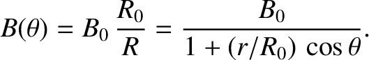
 is the toroidal magnetic field-strength on the magnetic axis (i.e., ,
  ). Note that the overall magnetic field-strength
varies slightly around the flux-surface, being larger at smaller major radii, and vice versa.
). Note that the overall magnetic field-strength
varies slightly around the flux-surface, being larger at smaller major radii, and vice versa.
Let us suppose that the parallel
(to the magnetic field) electric field-strength,
 , is comparatively weak, as is indeed the case in a high-temperature tokamak
plasma (otherwise the field would generate an absurdly large parallel current). (See Section 2.9.) If this is the case then (neglecting collisions, for the moment) our charged particle
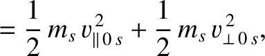
drifts around the magnetic flux-surface with a constant kinetic energy (recall that a magnetic field cannot do work on the particle). In other words,
, is comparatively weak, as is indeed the case in a high-temperature tokamak
plasma (otherwise the field would generate an absurdly large parallel current). (See Section 2.9.) If this is the case then (neglecting collisions, for the moment) our charged particle
drifts around the magnetic flux-surface with a constant kinetic energy (recall that a magnetic field cannot do work on the particle). In other words,
 is the particle's parallel velocity. However, the particle's magnetic moment, which is defined in Equation (2.73),
is also a constant of the motion. Equations (2.73) and (2.77) can be combined to give
is the particle's parallel velocity. However, the particle's magnetic moment, which is defined in Equation (2.73),
is also a constant of the motion. Equations (2.73) and (2.77) can be combined to give
![$\displaystyle v_{\parallel \,s}(\theta)= \pm \left(\frac{2}{m_s}\left[K_s-\mu_s\,B(\theta)\right]\right)^{1/2}.$](img698.png) |
(2.78) |
 (because
 clearly cannot be imaginary). In fact, if the
particle reaches a so-called bounce point, characterized by
clearly cannot be imaginary). In fact, if the
particle reaches a so-called bounce point, characterized by
 , where
 , then its parallel motion must reverse direction (i.e., the sign in the previous equation must flip).
Let
 and
and
 be the particle's parallel and perpendicular velocities at the outermost point of the flux-surface (i.e.,
  ), where the
magnetic field is weakest. It follows that
), where the
magnetic field is weakest. It follows that  and
and  both take the constant values
 |
 |
(2.79) |
 |
 |
(2.80) |
![$\displaystyle \frac{v_{\parallel\,s}(\theta)}{\vert v_{\parallel\,0\,s}\vert} =...
...{v_{\parallel\,0\,s}^{\,2}}\left[1 -\frac{B(\theta)}{B(0)}\right]\right)^{1/2}.$](img712.png) |
(2.81) |
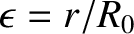 is the inverse aspect-ratio of the flux-surface, and we have made use of the large aspect-ratio approximation
 .
.
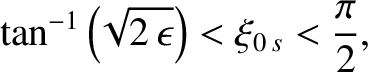
The previous equation, combined with the requirement that
 not be imaginary, leads to the conclusion that (neglecting collisions) there are two populations of charged particle on a magnetic flux-surface. The first population
satisfies
not be imaginary, leads to the conclusion that (neglecting collisions) there are two populations of charged particle on a magnetic flux-surface. The first population
satisfies
 |
(2.83) |
 , where
(See Figure 2.2.)
Assuming that the charged particles at the outermost point on the flux-surface have a Maxwellian velocity distribution, all possible values of
, where
(See Figure 2.2.)
Assuming that the charged particles at the outermost point on the flux-surface have a Maxwellian velocity distribution, all possible values of
 are equally likely. Thus, we conclude that the fraction of the particles on the flux-surface that are trapped is
[A more exact expression for
are equally likely. Thus, we conclude that the fraction of the particles on the flux-surface that are trapped is
[A more exact expression for  is specified in Equation (2.202).]
Given that
is specified in Equation (2.202).]
Given that
 , it is clear that the trapped particle fraction grows as we move from the innermost (i.e.,
  ) to the outermost (i.e.,
  ) magnetic flux-surface in the plasma.
Consider a trapped particle oscillating between bounce points located at
. Because the particle is drifting parallel to the magnetic field, its motion
is characterized by
 . [See Equation (1.76).] Let
  represent path-length along a magnetic field-line. It
follows that
represent path-length along a magnetic field-line. It
follows that
 . The particle's parallel equation of motion is
 |
(2.91) |
 for a trapped particle. Obviously, Equation (2.90)
has the same form as the equation of motion of a simple pendulum.
It follows that a deeply trapped particle, characterized by
for a trapped particle. Obviously, Equation (2.90)
has the same form as the equation of motion of a simple pendulum.
It follows that a deeply trapped particle, characterized by
 , executes simple harmonic motion in ,
between bounce points located at
, at the angular frequency
, executes simple harmonic motion in ,
between bounce points located at
, at the angular frequency
 .
In this case, the appropriate solution of Equation (2.90) is
A more accurate expression for the bounce frequency, which does not assume that the particle is deeply trapped, is
.
In this case, the appropriate solution of Equation (2.90) is
A more accurate expression for the bounce frequency, which does not assume that the particle is deeply trapped, is
![$\displaystyle \omega_{b\,s}(\theta_b) = \frac{\omega_{b\,s}}{(2/\pi)\,K(\sin[\theta_b/2])},$](img736.png) |
(2.93) |
 is a complete elliptic integral of the first kind [1].
Note that the bounce frequency decreases with increasing amplitude of the angular motion, eventually approaching zero
logarithmically as
is a complete elliptic integral of the first kind [1].
Note that the bounce frequency decreases with increasing amplitude of the angular motion, eventually approaching zero
logarithmically as
 .
.
Let us now take collisions into account. In the absence of collisions, the value of the pitch angle on the outboard midplane,
, is a constant of a given particle's
motion. Thus, we conclude that if the particle is initially trapped then it remains trapped at all subsequent times. However, collisions cause the
value of
to diffuse in velocity space. (Note that Coulomb collisions in a high temperature plasma are dominated by
small-angle scattering events [18], which means that each collision only causes a small change in
.)
It takes a time of order  (where is the collision time) to change
by order unity.
However, it is only necessary to change
by order
(where is the collision time) to change
by order unity.
However, it is only necessary to change
by order
 in order to de-trap a trapped particle. [See Equation (2.85).] The time
required for collisional de-trapping is thus
in order to de-trap a trapped particle. [See Equation (2.85).] The time
required for collisional de-trapping is thus
 then a trapped particle is collisionally de-trapped long before it has time to complete an oscillation between its
bounce points. Obviously, in this case, the plasma is sufficiently collisional that it is meaningless to draw a distinction between trapped and passing particles.
On the other hand, if
then a trapped particle is collisionally de-trapped long before it has time to complete an oscillation between its
bounce points. Obviously, in this case, the plasma is sufficiently collisional that it is meaningless to draw a distinction between trapped and passing particles.
On the other hand, if
 then collisions are too infrequent to interfere with the oscillations of a trapped particle between
its bounce points.
then collisions are too infrequent to interfere with the oscillations of a trapped particle between
its bounce points.
It is helpful to define the dimensionless collisionality parameter [64],
Note that .
It follows that the criterion for species- trapped particles to exist is
.
It follows that the criterion for species- trapped particles to exist is
 .
Table 2.4 shows that
.
Table 2.4 shows that
 and
and
 are both much less than unity in a tokamak fusion reactor, implying that populations of
trapped electrons as well as trapped ions exist in such reactors. Moreover, it is clear that the fraction of trapped particles, which is the same for both plasma species, is about
are both much less than unity in a tokamak fusion reactor, implying that populations of
trapped electrons as well as trapped ions exist in such reactors. Moreover, it is clear that the fraction of trapped particles, which is the same for both plasma species, is about  on the
outermost magnetic flux-surfaces.
on the
outermost magnetic flux-surfaces.
![\includegraphics[width=.8\textwidth]{Chapter02/Figure2_2.eps}](img769.png)
|
Let us examine the motion of a trapped particle slightly more accurately. In an axisymmetric tokamak plasma, the gyro-averaged motion of the particle takes place at constant toroidal canonical angular momentum:
where denotes magnetic vector potential.
Note that
Suppose that the particle is trapped on a magnetic flux-surface of minor radius
denotes magnetic vector potential.
Note that
Suppose that the particle is trapped on a magnetic flux-surface of minor radius  . We can write
in the immediate vicinity of the flux-surface, where use has been made of Equation (2.97). Now,
. We can write
in the immediate vicinity of the flux-surface, where use has been made of Equation (2.97). Now,
![$\displaystyle v_{\varphi\,s}\simeq v_{\parallel\,s} = \pm\sqrt{2\,\epsilon}\,\v...
...eft(\frac{\theta_b}{2}\right)-\sin^2\left(\frac{\theta}{2}\right)\right]^{1/2},$](img775.png) |
(2.99) |
 |
(2.100) |
for a trapped particle. Note that the  signs in Equation (2.101) correspond to motion in the
 and
and
 directions, respectively. As is illustrated in Figure 2.2, a trapped particle that oscillates between its
bounce points makes radial excursions from the guiding magnetic flux-surface that are of amplitude
directions, respectively. As is illustrated in Figure 2.2, a trapped particle that oscillates between its
bounce points makes radial excursions from the guiding magnetic flux-surface that are of amplitude
 . In fact, the gyro-averaged orbit's poloidal cross-section looks a
little like a banana. Hence, such orbits are known as banana orbits, and
. In fact, the gyro-averaged orbit's poloidal cross-section looks a
little like a banana. Hence, such orbits are known as banana orbits, and
 is known as the banana width [52]. [Note that
is the banana width of a barely trapped particle (i.e.,
is known as the banana width [52]. [Note that
is the banana width of a barely trapped particle (i.e.,
 ). Deeply
trapped particles (i.e.,
) have much narrower banana widths.] Finally, as is clear from Tables 2.1 and 2.4, although the electron and
ion banana widths in a tokamak fusion reactor are much greater than the corresponding gyro-radii, they are much smaller than the minor radius of the plasma.
). Deeply
trapped particles (i.e.,
) have much narrower banana widths.] Finally, as is clear from Tables 2.1 and 2.4, although the electron and
ion banana widths in a tokamak fusion reactor are much greater than the corresponding gyro-radii, they are much smaller than the minor radius of the plasma.
![$\displaystyle \frac{v_{\parallel\,s}(\theta)}{\vert v_{\parallel\,0\,s}\vert}\s...
...l\,0\,s}^{\,2}}\,2\,\epsilon\,\sin^2\left(\frac{\theta}{2}\right)\right]^{1/2},$](img713.png)

![$\displaystyle \frac{ds}{dt} = v_{\parallel\,s} = \pm\vert v_{\parallel\,0\,s}\vert\left[1- \frac{\sin^2(\theta/2)}{\sin^2(\theta_b/2)}\right]^{1/2},$](img728.png)
![$\displaystyle \frac{d\theta}{dt} =\pm \frac{\vert v_{\parallel\,0\,s}\vert}{q\,R_0} \left[1- \frac{\sin^2(\theta/2)}{\sin^2(\theta_b/2)}\right]^{1/2}.$](img729.png)


![$\displaystyle r= r_b \pm{\rm sgn}(e_s)\, \rho_{b\,s}\left[\sin^2\left(\frac{\theta_b}{2}\right)-\sin^2\left(\frac{\theta}{2}\right)\right]^{1/2},$](img777.png)