Lowest-Order Flows
To lowest order in the small parameter
 , Equations (2.116) and (2.118) yield
| 0 |
 |
(2.132) |
| 0 |
![$\displaystyle \simeq \frac{e_s}{m_s}\left[\frac{5}{2}\,p_s\,({\bf E}_\perp+{\bf...
...}_s\times {\bf B}\right]
-\nabla\left(\frac{5}{2}\,\frac{T_s\,p_s}{m_s}\right).$](img857.png) |
(2.133) |
 ).
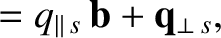
The first term on the right-hand side of Equation (2.136) is the E-cross-B velocity,
).
The first term on the right-hand side of Equation (2.136) is the E-cross-B velocity,
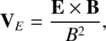 |
(2.138) |
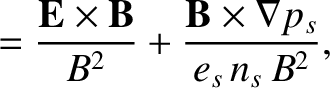
that is common to all plasma species [18]. The second term
is the diamagnetic velocity,
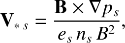 |
(2.139) |
which is different for electrons and ions, and is a consequence of the rapid gyro-motions of charged particles in the presence of equilibrium pressure gradients [18]. The drift ordering (2.113) ensures
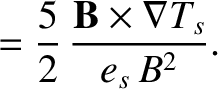
that the E-cross-B and diamagnetic velocities are similar in magnitude. It is clear from Equation (2.137) that there is a diamagnetic flow of heat, as well as particles, around flux-surfaces; this heat flow is the same as that
associated with the cross thermal conductivities introduced in Section 2.6.
To lowest order in the small parameter
, Equations (2.115) and (2.117) yield
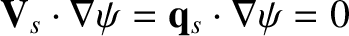
Here, use has been made of
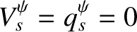
 . Clearly, the
lowest-order particle and heat flows are both divergence free. Now, the fact that
implies that
. Clearly, the
lowest-order particle and heat flows are both divergence free. Now, the fact that
implies that
 . Making use of these results, the previous two equations can be combined with Equations (2.123) and (2.126), as well as the fact that
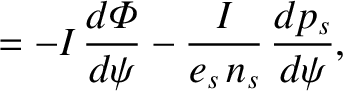
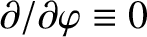 in an axisymmetric equilibrium, to give [34]
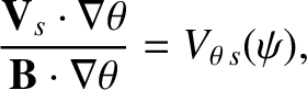 |
(2.142) |
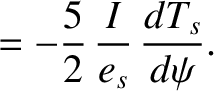
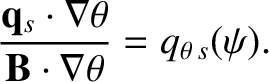 |
(2.143) |
 , we obtain
where
Here, use has been made of Equations (2.136) and (2.137).
, we obtain
where
Here, use has been made of Equations (2.136) and (2.137).