Calculation of Inductance Matrix

In principle, we could determine the relationship between ${\mit\Delta\Psi}_k$ and the ${\mit\Psi}_k$ (which is equivalent to determining the relationship between the $I_k$ and the ${\mit\Phi}_k$) by solving Equations (14.46) and (14.47) subject to suitable spatial boundary conditions at $r=0$ and $r=r_{100}$ [11,14,22]. However, in this chapter, we shall adopt a more direct approach [12,13,15,16].

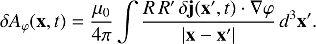
According to the Biot-Savart law [27]:

$$\delta A_{\varphi}({\bf x},t) = \frac{\mu_0}{4\pi}\int \frac{R\,R... ...f j}({\bf x'},t)\cdot\nabla\varphi}{\vert{\bf x}-{\bf x}'\vert}\,d^{3}{\bf x}'.$$ (14.102)

Let us assume that

$$\delta A_\varphi (R,\varphi,Z,t) = \delta A_\varphi(R,0,Z,t)\,{\rm e}^{-{\rm i}\,n\,\varphi}.$$ (14.103)

It follows that we can evaluate the integral on the right-hand side of Equation (14.102) at $\varphi=0$ without loss of generality. Now,

$$\delta {\bf j}(R',\varphi',Z',t)\cdot\nabla\varphi= \delta j^{\,\varphi}(R',0,Z',t)\,{\rm e}^{-{\rm i}\,n\,\varphi'}\cos\varphi',$$ (14.104)

so we get

$$\delta A_\varphi(R,0,Z,t)= \frac{\mu_0}{4\pi}\int_0^\infty \oint R\,R'\,\delta j^{\,\varphi}(R',0,Z',t)\,G(R,Z;R',Z')\,{\cal J}'\,dr'\,d\theta',$$ (14.105)

where

$$G(R,Z;R',Z') = \frac{1}{2}\oint \frac{\left(\cos[(n-1)\,\varphi']... ...arphi'}{\left[R^{2}+R'^{\,2} +(Z-Z')^{2} -2\,R\,R'\,\cos\varphi'\right]^{1/2}}.$$ (14.106)

Finally, making use of the standard definition of a toroidal function [23],

$$P^{\,n}_{-1/2}(\cosh\eta) =\frac{(-1)^{n}\,{\mit\Gamma}(1/2)\,{\m... ...nt \frac{\cos(n\,\varphi)\,d\varphi}{(\cosh\eta-\sinh\eta\,\cos\varphi)^{1/2}},$$ (14.107)

where ${\mit\Gamma}(x)$ denotes a gamma function [1], we arrive at

$$G(R,Z;R',Z') = \frac{(-1)^{n+1}\,\pi^{2}}{{\mit\Gamma}(1/2)\,{\mit\Gamma}(n+1/2)} \left[\frac{\cosh\eta}{R^{2}+R'^{\,2}+(Z-Z')^{2}}\right]^{1/2}$$

$$\phantom{=}\times\left[(n-1/2)\,P_{-1/2}^{\,n-1}(\cosh\eta)+ \frac{P_{-1/2}^{\,n+1}(\cosh\eta)}{n+1/2}\right],$$ (14.108)

where

$$\eta = \tanh^{-1}\left[\frac{2\,R\,R'}{R^{2}+R'^{\,2}+(Z-Z')^{2}}\right].$$ (14.109)

According to Equations (14.60) and (14.66),

$${\cal J}\,\mu_0\,\delta j^{\,\varphi}(r,\theta,0,t)=-\sum_{k=1,K} {\mit\Delta\Psi}_k(t)\,\delta (r-r_k)\,{\rm e}^{\,{\rm i}\,m_k\,\theta}.$$ (14.110)

Furthermore, Equations (14.65) and (14.78) yield

$${\mit\Psi}_k(t) = \frac{1}{R_0}\oint \delta A_{\varphi}(r_k,\theta,0,t)\,{\rm e}^{-{\rm i}\,m_k\,\theta}\,\frac{d\theta}{2\pi}.$$ (14.111)

Hence, combining the previous two expressions with Equation (14.105), we obtain the expected normalized inductance relation [see Equation (14.94)],

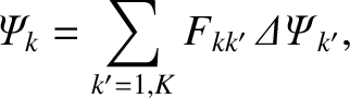$${\mit\Psi}_k = \sum_{k'=1,K} F_{kk'}\,{\mit\Delta\Psi}_{k'},$$ (14.112)

for $k=1,K$, where [12,13,15,16]

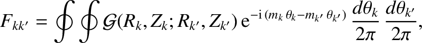$$F_{kk'} = \oint\oint {\cal G}(R_k,Z_k;R_{k'},Z_{k'})\,{\rm e}^{-{... ...eta_k-m_{k'}\,\theta_{k'})}\,\frac{d\theta_k}{2\pi}\,\frac{d\theta_{k'}}{2\pi},$$ (14.113)

and

$${\cal G}(R_k,Z_k;R_{k'},Z_{k'}) = \frac{(-1)^{n}\,\pi^{2}\,R_k\,R_{k'}/R_0}{2\,{\mit\Gamma}(1/2)\... ...ft[\frac{\cosh\eta_{kk'}}{R_k^{\,2}+R_{k'}^{\,2}+(Z_k-Z_{k'})^{2}}\right]^{1/2}$$

$$\phantom{=}\times\left[(n-1/2)\,P_{-1/2}^{\,n-1}(\cosh\eta_{kk'})+ \frac{P_{-1/2}^{\,n+1}(\cosh\eta_{kk'})}{n+1/2}\right],$$ (14.114)

with

$$\eta_{kk'} = \tanh^{-1}\left[\frac{2\,R_k\,R_{k'}}{R_k^{\,2}+R_{k'}^{\,2}+(Z_k-Z_{k'})^{2}}\right].$$ (14.115)

Here, $k$ and $k'$ index the various rational surfaces in the plasma. Moreover, the double integral in Equation (14.113) is taken around the $k$th rational surface (cylindrical coordinates $R_k$, 0, $Z_k$; flux coordinates $r_k$, $\theta_k$, 0, with $r_k$ constant; resonant poloidal mode number $m_k$) and the $k'$th rational surface (cylindrical coordinates $R_{k'}$, 0, $Z_{k'}$; flux coordinates $r_{k'}$, $\theta_{k'}$, 0, with $r_{k'}$ constant; resonant poloidal mode number $m_{k'}$).

Note that

$${\cal G} (R_{k'},Z_{k'};R_k,Z_k) = {\cal G}(R_k,Z_k;R_{k'},Z_{k'}),$$ (14.116)

which, from Equation (14.113), implies that the F-matrix is Hermitian [see Equation (14.100)], as must be the case.

Finally, according to Equations (14.95) and (14.113), the unnormalized inductance matrix takes the form

$$L_{kk'} =\mu_0\,R_0 \oint\oint {\cal G}(R_k,Z_k;R_{k'},Z_{k'})\,{... ...eta_k-m_{k'}\,\theta_{k'})}\,\frac{d\theta_k}{2\pi}\,\frac{d\theta_{k'}}{2\pi}.$$ (14.117)

The Hermitian L-matrix, $L_{kk'}$, specifies the self and mutual inductances of the helical current sheets that flow at the various rational surfaces within the plasma.

Note that the calculation of the F-matrix outlined in this section is only approximate. The exact calculation is specified in References [11] and [22].