The analysis of Section 5.16 suggests that a non-zero value of the reconnected magnetic flux at the  th rational surface,
 , will cause
a helical magnetic island chain, with
, will cause
a helical magnetic island chain, with  periods in the poloidal direction, and
  periods in the toroidal direction, to open in the immediate vicinity of the surface. Let us investigate the properties of such a chain.
We can write
 |
(14.71) |
where
 |
(14.72) |
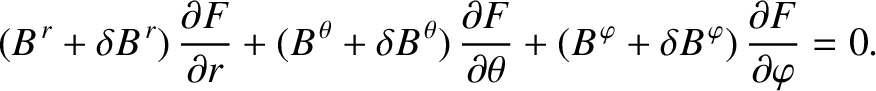
Suppose that all terms in the previous equation are of equal importance. It follows from Equation (14.13) that
 |
(14.73) |
and, hence, that
 |
(14.74) |
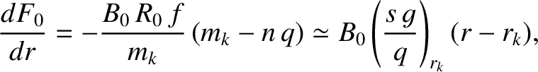
Thus, Equations (14.14)–(14.16) and (14.71) yield
where the neglected terms are, at least, of order
 smaller than the retained terms. The previous three equations are consistent with Equations (14.44), (14.51), and (14.52) provided that
 |
(14.78) |
Let us search for a function,
 , which is such that
 |
(14.79) |
It follows from Equations (14.2), (14.4), and (14.6) that
 |
(14.80) |
Equations (14.3), (14.19)–(14.21), and (14.75)–(14.77) yield
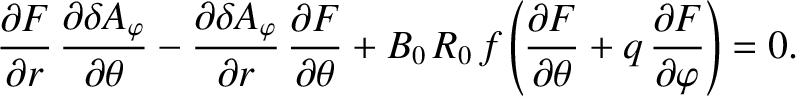 |
(14.81) |
Suppose that
 |
(14.82) |
The previous two equations give
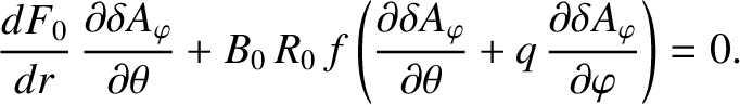 |
(14.83) |
According to Equation (14.78), we can write
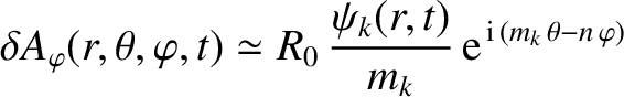 |
(14.84) |
in the vicinity of the th rational surface, where we have neglected the non-resonant components of
 (because we do not expect them to open up an island chain at this surface) [26]. The previous two
equations yield
(because we do not expect them to open up an island chain at this surface) [26]. The previous two
equations yield
 |
(14.85) |
where
 is the magnetic shear, and use has been made of Equation (14.18), as well as the fact that
 .
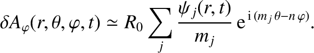
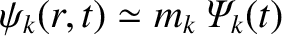
Finally, Equations (14.65), (14.82), (14.84), and (14.85) can be combined to give
.
Finally, Equations (14.65), (14.82), (14.84), and (14.85) can be combined to give
 |
(14.86) |
where
 . Here, we have taken the (physical) real part of
  , and use has been made of the constant-
 approximation that
 in the immediate vicinity of the th rational surface. (See Chapter 5.)
The previous equation can be written
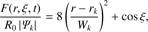 |
(14.87) |
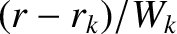
where
![$\displaystyle W_k = 4\,R_0\left[\left(\frac{q}{g\,s}\right)_{r_k}\,\frac{\vert{\mit\Psi}_k\vert}{B_0\,R_0}\right]^{1/2}.$](img4142.png) |
(14.88) |
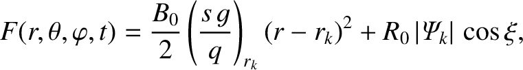
Now, according to Equation (14.79), the contours of the function
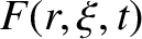 map out the perturbed magnetic flux-surfaces in the
immediate vicinity of the th rational surface. These contours are shown in Figure 5.7 [with
map out the perturbed magnetic flux-surfaces in the
immediate vicinity of the th rational surface. These contours are shown in Figure 5.7 [with
 playing the
role of
playing the
role of
 ]. It can be seen that the reconnected magnetic flux at the th rational surface has indeed opened up
a helical magnetic island chain, with periods in the poloidal direction, and periods in the toroidal direction, at the surface. Moreover, the full radial width of the island chain (in
]. It can be seen that the reconnected magnetic flux at the th rational surface has indeed opened up
a helical magnetic island chain, with periods in the poloidal direction, and periods in the toroidal direction, at the surface. Moreover, the full radial width of the island chain (in  ) is
) is  . Incidentally, the previous
equation is the toroidal generalization of the cylindrical result, (5.129).
. Incidentally, the previous
equation is the toroidal generalization of the cylindrical result, (5.129).