Next: Plasma Rotation Up: Linear Resonant Response Model Previous: Response Regimes in Tokamak Contents
 limit, the solution to this equation takes the form
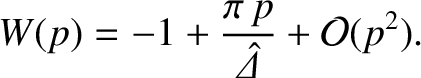
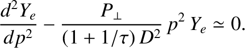
[See Equation (5.83).] In the large- limit, Equations (5.78)–(5.81) reduce to
This is a parabolic cylinder equation [1] whose most general large- solution is
where
limit, the solution to this equation takes the form
[See Equation (5.83).] In the large- limit, Equations (5.78)–(5.81) reduce to
This is a parabolic cylinder equation [1] whose most general large- solution is
where  and
and  are arbitrary constants,
and
are arbitrary constants,
and
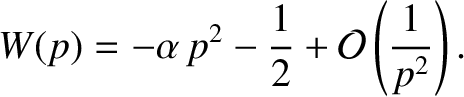
![$\displaystyle \alpha =\left[\frac{P_\perp}{(1+1/\tau)\,D^2}\right]^{1/2}.$](img2301.png) |
(5.118) |
. Hence, we
must select  in Equation (5.117), which implies that
at large .
in Equation (5.117), which implies that
at large .
![\includegraphics[width=1.\textwidth]{Chapter05/Figure5_5.eps}](img2304.png)
|
Let us make use of the so-called Riccati transformation [5,18],
 |
(5.120) |
behavior of the solution to the previous equation is
Likewise, according to Equation (5.119), the large- behavior of the solution is
Equation (5.121) is conveniently solved numerically by launching a solution of the form (5.123) at large , and then
integrating backward to small [18]. Equation (5.122) yields
 |
(5.124) |
Figure 5.5 shows a numerical solution of the resonant layer equation for a low-field tokamak
fusion reactor. This calculation is made with
 ,
,  ,
,
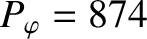 ,
,
 , and
, and  , assuming that
  is real. (See Table 5.1.) Note that
 parameterizes the amplitude and phase of
a shielding current that is driven inductively at the rational surface, in response to a rotating tearing perturbation in the
outer region, and acts to suppress magnetic reconnection at the surface [11]. It can be seen that
the shielding current is zero when
parameterizes the amplitude and phase of
a shielding current that is driven inductively at the rational surface, in response to a rotating tearing perturbation in the
outer region, and acts to suppress magnetic reconnection at the surface [11]. It can be seen that
the shielding current is zero when  , which is equivalent to
 . In other words, the shielding current is zero when the tearing perturbation in the outer region
rotates at the frequency of a naturally unstable tearing mode at the rational surface [2,11]. (See Chapter 6.) The shielding
current clearly increases linearly with
. In other words, the shielding current is zero when the tearing perturbation in the outer region
rotates at the frequency of a naturally unstable tearing mode at the rational surface [2,11]. (See Chapter 6.) The shielding
current clearly increases linearly with  when
when
 , but saturates in magnitude as
 .
.
![\includegraphics[width=1.\textwidth]{Chapter05/Figure5_6.eps}](img2318.png)
|
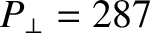
Figure 5.6 shows a numerical solution of the resonant layer equation for a high-field tokamak
fusion reactor. This calculation is made with
 ,
,  ,
,
, and , assuming that is real. (See Table 5.1.) Note that the figure is very similar to Figure 5.5, indicating that the resonant layer responses in low-field and high-field tokamak fusion reactors do not differ substantially from one another.
,
,
, and , assuming that is real. (See Table 5.1.) Note that the figure is very similar to Figure 5.5, indicating that the resonant layer responses in low-field and high-field tokamak fusion reactors do not differ substantially from one another.
![$\displaystyle Y_e(p)\rightarrow Y_0\left[\frac{\skew{6}\hat{\mit\Delta}}{\pi\,p} + 1+ {\cal O}(p)\right].$](img2297.png)
![$\displaystyle Y_e(p) = \frac{A\,{\rm e}^{-\alpha\,p^2/2} + B\,{\rm e}^{+\alpha\,p^2/2}}{p^{1/2}}\left[1+{\cal O}\left(\frac{1}{p^2}\right)\right],$](img2299.png)
![$\displaystyle Y_e(p) = \frac{A\,{\rm e}^{-\alpha\,p^2/2} }{p^{1/2}}\left[1+{\cal O}\left(\frac{1}{p^2}\right)\right],$](img2303.png)

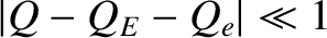
![$\displaystyle \frac{dW}{dp} = \left[\frac{2\,p}{-{\rm i}\,(Q-Q_E-Q_e)+ p^2}-\fr...
...- \frac{W^{\,2}}{p} + p\left[-{\rm i}\,(Q-Q_E-Q_e)+p^2\right]\frac{B(p)}{C(p)}.$](img2306.png)