Fourier Transformation

Equations (5.57)–(5.60) are most conveniently solved in Fourier transform space [7,15,18]. Let

$$\skew{3}\bar{\phi}(p) = \int_{-\infty}^\infty \skew{3}\tilde{\phi}(X)\,{\rm e}^{-{\rm i}\,p\,X}\,dX,$$ (5.72)

et cetera. The Fourier transformed layer equations become

$$-{\rm i}\,(Q-Q_E-\,Q_{e})\,\bar{\psi} =\frac{d}{dp}\!\left(\skew{3}\bar{\phi}-\bar{N}\right) -p^2\,\bar{\psi},$$ (5.73)

$$-{\rm i}\,(Q-Q_E)\,\bar{N} = - {\rm i}\,Q_{e}\,\skew{3}\bar{\phi} + c_\beta^{\,2}\,\frac{d\bar{V}}{dp}-D^{2}\,\frac{d(p^2\,\bar{\psi})}{dp} - P_\perp\,p^2\bar{N},$$ (5.74)

$$-{\rm i}\,(Q-Q_E -Q_{i})\,p^2\,\skew{3}\bar{\phi} = \frac{d(p^2\,\bar{\psi})}{dp}- P_\varphi\,p^4 \left(\skew{3}\bar{\phi} + \frac{\bar{N}}{\tau}\right),$$ (5.75)

$$-{\rm i}\,(Q-Q_E)\,\bar{V} = {\rm i}\,Q_{e}\,\bar{\psi} +\frac{d\bar{N}}{dp}- P_\varphi\,p^2\,\bar{V},$$ (5.76)

where, for a tearing parity solution [10],

$$\skew{3}\bar{\phi}(p)\rightarrow \skew{3}\bar{\phi}_0 \left[\frac{\skew{6}\hat{\mit\Delta}}{\pi\,p} + 1+ {\cal O}(p)\right]$$ (5.77)

as $p\rightarrow 0$. Here, $\skew{3}\bar{\phi}_0$ is an arbitrary constant, and use has been made of Equation (5.71).

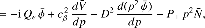
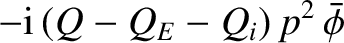
In accordance with our previous discussion, we have neglected the parallel transport terms in Equation (5.74). Let us also ignore the term $c_\beta^{\,2}\,d\bar{V}/dp$. This approximation can be justified a posteriori. It is equivalent to the neglect of the contribution of ion parallel dynamics to the linear plasma response in the resonant layer, and effectively decouples Equation (5.76) from Equations (5.73)–(5.75) [22]. Equations (5.73)–(5.75) reduce to [7,15]

$$\frac{d}{dp}\!\left[A(p)\,\frac{dY_e}{dp}\right] - \frac{B(p)}{C(p)}\,p^{2}\,Y_e = 0,$$ (5.78)

where

$$A(p) = \frac{p^2}{-{\rm i}\,(Q-Q_E-Q_e)+ p^2},$$ (5.79)

$$B(p) = -(Q-Q_E)\,(Q-Q_E-Q_i)-{\rm i}\,(Q-Q_E-Q_i)\,(P_\varphi+P_\perp)\,p^2 + P_\varphi\,P_\perp\,p^4,$$ (5.80)

$$C(p) = -{\rm i}\,(Q-Q_E-Q_e) +\left[P_\perp - {\rm i}\,(Q-Q_E-Q_i)\,D^2\right] p^2+(1+1/\tau)\,P_\varphi\,D^2\,p^4,$$ (5.81)

and $Y_e=\skew{3}\bar{\phi} - \bar{N}$ is the normalized, Fourier transformed, electron fluid stream-function. It is easily demonstrated that

$$Y_e(p)\rightarrow \left(\frac{Q-Q_E-Q_e}{Q-Q_E}\right)\skew{3}\bar{\phi}(p)$$ (5.82)

as $p\rightarrow 0$. Hence, the boundary conditions on Equation (5.78) are that $Y_e(p)$ is bounded as $p\rightarrow\infty$, and

$$Y_e(p)\rightarrow Y_0\left[\frac{\skew{6}\hat{\mit\Delta}}{\pi\,p} + 1+ {\cal O}(p)\right]$$ (5.83)

as $p\rightarrow 0$, where $Y_0$ is an arbitrary constant. Here, use has been made of Equation (5.77). In the following, we shall assume that $\vert Q\vert\sim \vert Q_E\vert\sim Q_\ast$, $P_\varphi\sim P_\perp \sim P$, and $\tau\sim {\cal O}(1)$, for the sake of simplicity.