Constant-$\psi$ Limit

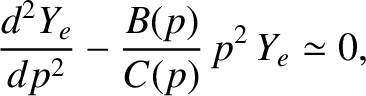
Let us suppose that there are two layers in $p$ space. In the small-$p$ layer, suppose that Equation (5.78) reduces to

$$\frac{d}{dp}\!\left[\frac{p^2}{-{\rm i}\,(Q-Q_E-Q_e) + p^2}\,\frac{dY_e}{dp}\right]\simeq 0$$ (5.84)

when $p\sim Q^{1/2}$. Integrating directly, we find that

$$Y_e(p) \simeq Y_0 \left\{\frac{\skew{6}\hat{\mit\Delta}}{\pi}\lef... ... + \frac{p}{{\rm i}\,(Q-Q_E-Q_e)}\right] + 1 + {\cal O}\left(p^2\right)\right\}$$ (5.85)

for $p\lesssim {\cal O}(Q^{1/2})$, where use has been made of Equation (5.83). The two-layer approximation is equivalent to the well-known constant-$\psi$ approximation [17].

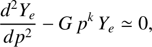
In the large-$p$ layer, for $p\gg {\cal O}(Q^{1/2})$, we obtain

$$\frac{d^2 Y_e}{dp^2} - \frac{B(p)}{C(p)}\,p^2\,Y_e\simeq 0,$$ (5.86)

with $Y_e(p)$ bounded as $p\rightarrow\infty$. Asymptotic matching to the small-$p$ layer solution (5.85) yields the boundary condition

$$Y_e(p)\simeq Y_0\left[1+ \frac{\skew{6}\hat{\mit\Delta}}{\pi}\,\frac{p}{{\rm i}\,(Q-Q_E-Q_e)}+ {\cal O}\left(p^2\right)\right]$$ (5.87)

as $p\rightarrow 0$.

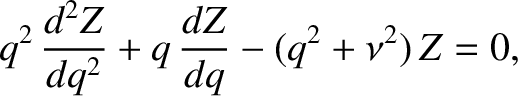
In the various constant-$\psi$ linear response regimes considered in Section 5.9, Equation (5.86) reduces to an equation of the form

$$\frac{d^2Y_e}{dp^2}- G\,p^k\,Y_e\simeq 0,$$ (5.88)

where $k$ is real and non-negative, and $G$ is a complex constant. Let $Y_e=\!\sqrt{p}\,Z$ and $q=\!\sqrt{G}\,p^j/j$, where $j=(k+2)/2$. The previous equation transforms into a modified Bessel equation of general order,

$$q^2\,\frac{d^2Z}{dq^2} + q\,\frac{dZ}{dq} - (q^2+\nu^2)\,Z =0,$$ (5.89)

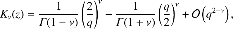
where $\nu=1/(k+2)$. The solution that is bounded as $q\rightarrow \infty$ has the small-$q$ expansion [1]

$$K_\nu(z)= \frac{1}{{\mit\Gamma}(1-\nu)}\left(\frac{2}{q}\right)^\... ...it\Gamma}(1+\nu)}\left(\frac{q}{2}\right)^\nu + {\cal O}\left(q^{2-\nu}\right),$$ (5.90)

where ${\mit\Gamma}(z)$ is a gamma function. A comparison of this expression with Equation (5.87) reveals that

$$\skew{6}\hat{\mit\Delta} = \frac{\nu^{2\nu-1}\,\pi\,{\mit\Gamma}(... ...u)}{{\mit\Gamma}(\nu)}\left[-{\rm i}\,\left(Q-Q_E-\,Q_e\right)\right]G^{\,\nu}.$$ (5.91)

Note, finally, that $p_\ast\sim \vert G\vert^{-\nu}$, where $p_\ast$ denotes the width of the large-$p$ layer in $p$ space. This width must be larger than $Q^{1/2}$ (i.e., the width of the small-$p$ layer) in order for the constant-$\psi$ approximation to hold. Finally, it is easily demonstrated that the neglect of the term involving $c_\beta$ in Equation (5.74) is justified provided that $c_\beta\ll (Q+P\,p_\ast^2)^{1/2}\,p_\ast$.