Consider an equilibrium magnetic flux-surface whose label is  .
Let
.
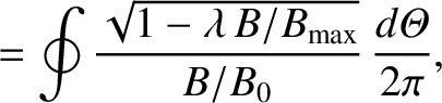
Let
 |
(A.8) |
where
 , and
, and  is the equilibrium magnetic field. Here,
  ,
,  ,
,  ,
,  ,
,  , and
, and  are specified in Sections 14.2 and 14.4.
It is helpful to define a new poloidal angle
are specified in Sections 14.2 and 14.4.
It is helpful to define a new poloidal angle
 such that
 |
(A.9) |
Let
 |
 |
(A.10) |
 |
 |
(A.11) |
 |
 |
(A.12) |
 |
 |
(A.13) |
 |
 |
(A.14) |
 |
 |
(A.15) |
 is the maximum value of
  on the magnetic
flux-surface, and
on the magnetic
flux-surface, and  a positive integer.
The species-
a positive integer.
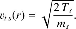
The species- transit frequency is written [7]
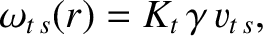 |
(A.16) |
where
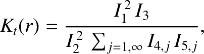 |
(A.17) |
and
 |
(A.18) |
Here,  is the
species- mass, and
is the
species- mass, and  the species- temperature (in energy units). The fraction of passing particles
is [7]
the species- temperature (in energy units). The fraction of passing particles
is [7]
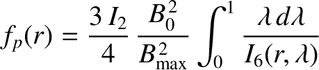 |
(A.19) |
[See Equation (2.200).]
Finally, the dimensionless species- collisionality parameter [see Equation (2.95)].
is written [7]
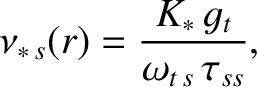 |
(A.20) |
where
[See Equation (2.190).]
Here, the Coulomb logarithm,
 [1], is assumed to take the same large constant value (i.e.,
 ),
independent of species.
),
independent of species.