Next: Ordering Scheme Up: Nonlinear Neoclassical Resonant Response Previous: Magnetic Field-Line Curvature Contents
 , in our reduced
neoclassical drift-MHD model equal to the minor radius of the rational surface,
, in our reduced
neoclassical drift-MHD model equal to the minor radius of the rational surface,  . It is also convenient to work in a frame of reference that co-rotates with the magnetic island chain that develops in the inner region. This goal can be achieved by making the transformation
 and
and
 , where
 is the rotation
frequency of the tearing mode in the laboratory frame. In the co-rotating reference frame, the
normalized reconnected flux at the rational surface,
is the rotation
frequency of the tearing mode in the laboratory frame. In the co-rotating reference frame, the
normalized reconnected flux at the rational surface,
 [see Equations (3.72) and (3.184)], is assumed to be a positive real quantity. It is helpful to define the reduced (by a factor four) radial width of the magnetic island chain:
 [see Equation (5.129)]. Here,
  is the plasma major radius (see Section 3.2), and
  is the magnetic shear-length at the rational surface [see Equation (5.27)].
As before (see Section 8.2), it is assumed that
 , where
  is the linear layer width. (See Chapter 6.)
In other words, the width of the island chain is assumed to be much greater than the linear layer width, but much less than the minor
radius of the rational magnetic flux-surface. Let
is the linear layer width. (See Chapter 6.)
In other words, the width of the island chain is assumed to be much greater than the linear layer width, but much less than the minor
radius of the rational magnetic flux-surface. Let
 . Reusing the analysis of Sections 5.3 and 8.2,
we find that
. Reusing the analysis of Sections 5.3 and 8.2,
we find that
 (i.e., many island widths from the rational surface).
Here,
(i.e., many island widths from the rational surface).
Here,
 ,
,
 ,
,
 ,
,
 , and
, and
 , where
  is the E-cross-B
velocity profile in the outer region [see Equation (5.21)],
is the E-cross-B
velocity profile in the outer region [see Equation (5.21)],  the diamagnetic velocity profile [see Equation (5.29)],
and
the diamagnetic velocity profile [see Equation (5.29)],
and  the magnetic shear profile [see Equation (5.28)].
Moreover,
the magnetic shear profile [see Equation (5.28)].
Moreover,
 ,
and
,
and
![$\hat{V}_E' = [r\,dV_E/dr]_{r_{s-}}^{r_{s+}}/V_A$](img3482.png) .
The parameter
.
The parameter
 is introduced into the analysis in order to take into account the fact that the E-cross-B velocity profile in the outer region (i.e., everywhere in the plasma apart from the immediate vicinity of the magnetic island chain) develops a
gradient discontinuity at the rational surface in response to the localized electromagnetic torque that emerges
at the surface. (See Section 8.2.) Note, finally, that in neglecting any dependance of
is introduced into the analysis in order to take into account the fact that the E-cross-B velocity profile in the outer region (i.e., everywhere in the plasma apart from the immediate vicinity of the magnetic island chain) develops a
gradient discontinuity at the rational surface in response to the localized electromagnetic torque that emerges
at the surface. (See Section 8.2.) Note, finally, that in neglecting any dependance of
 on
on  in Equation (11.58)
we are making use of the so-called constant-
in Equation (11.58)
we are making use of the so-called constant- approximation [9,19], which
is valid as long as
approximation [9,19], which
is valid as long as
 [4,6]. Here,
 is defined in Equations (3.73) and (3.183).
Equations (11.58)–(11.62) are analogous to the boundary conditions in our previous reduced non-neoclassical drift-MHD model, (8.2)–(8.6), apart from Equation (11.61). The latter equation is derived on the assumption that ion neoclassical poloidal flow damping relaxes the ion poloidal velocity profile to its neoclassical value (see Section 2.18) many island widths away from the rational surface.
Let
 and
and
 ,
where
,
where
 is the diamagnetic frequency at the rational surface [see Equation (5.47)], and
 .
It follows that
.
It follows that
 in the immediate vicinity of the island chain.
It is helpful to define the
rescaled fields
in the immediate vicinity of the island chain.
It is helpful to define the
rescaled fields
 ,
,
 ,
,
 ,
,
 , and
, and
 , where
Equations (11.50)–(11.56) rescale to give
Here, ,
,
 ,
and we have set
,
and we have set
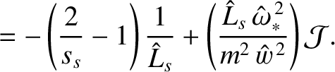
![$\displaystyle \hat{E}_\parallel =\left[ \left(\frac{2}{s_s}-1\right)\frac{1}{\hat{L}_s}+\alpha_{bs}\,\frac{\hat{V}_\ast}{\hat{d}_i}\right]\hat{\eta}_\parallel.$](img3498.png) |
(11.73) |
 is the effective pressure gradient scale-length at the rational surface [see Equation (8.35)],
 is the ion sound radius [see Equation 4.75)], and the dimensionless
quantities
is the ion sound radius [see Equation 4.75)], and the dimensionless
quantities
 ,
,
 ,
,
 ,
,
 ,
,
 ,
,
 , and
, and
 are defined in Section 8.3.
Equations (11.68)–(11.72) must be solved subject to the boundary conditions [see Equations (11.58)–(11.62) and (11.63)–(11.67)]
as . Here,
where
. Here,
where
 is the E-cross-B frequency at the rational surface.
Note that
is the E-cross-B frequency at the rational surface.
Note that
 ,
,  ,
,
 ,
,  , and
, and  are all
 quantities in the inner region.
Note, further, that the boundary conditions (11.83)–(11.87),
as well as the symmetry of the rescaled reduced neoclassical drift-MHD equations, (11.68)–(11.72), ensure that
, , and
are even functions of
quantities in the inner region.
Note, further, that the boundary conditions (11.83)–(11.87),
as well as the symmetry of the rescaled reduced neoclassical drift-MHD equations, (11.68)–(11.72), ensure that
, , and
are even functions of  , whereas and
are odd functions.
, whereas and
are odd functions.
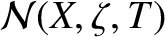
Finally, asymptotic matching between the inner region and the surrounding plasma yields (see Section 8.10)
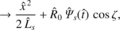
![$\displaystyle \rightarrow \left[\frac{\hat{\omega}}{m}- \hat{V}_E(\hat{t})\right]\hat{x} - \frac{\varsigma}{4}\,\hat{V}_E'(\hat{t})\,\hat{x}^{\,2},$](img2629.png)
![$\displaystyle \rightarrow \frac{q_s}{\epsilon_s}\left[\frac{\hat{\omega}}{m}-\h...
...a_i}{1+\eta_i}\right)-\frac{\varsigma}{2}\,\hat{V}_E'(\hat{t})\,\hat{x}\right],$](img3480.png)


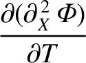


![$\displaystyle \phantom{=}-\epsilon_c\,\epsilon_\theta\left({\cal V} -\xi\,\part...
...{\cal N}\right]\right)+\epsilon_c\,\epsilon_\varphi\,\partial_X^{\,2} {\cal V},$](img3496.png)


![$\displaystyle =f_{t\,s}\,\xi\left[\beta_{11}\left(1-\alpha_1\,\frac{1}{1+\tau}\...
...ta_e}\right]\left(\frac{w}{d_\beta}\right)^2 = \left(\frac{w}{w_{bs}}\right)^2,$](img3505.png)

![$\displaystyle =f_{t\,s}\,\xi\left[\left(\beta_{11}+\frac{2}{5}\,\epsilon_1\righ...
...\eta_e}{1+\eta_e}-\frac{\alpha_2}{\tau'}\right]\left(\frac{w}{d_\beta}\right)^2$](img3507.png)

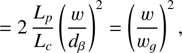

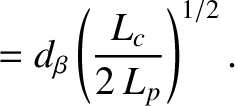
![$\displaystyle = d_\beta\left\{f_{t\,s}\,\xi\left[\beta_{11}\left(1-\alpha_1\,\f...
...
-\beta_{12}\,\frac{\tau}{1+\tau}\frac{\eta_e}{1+\eta_e}\right]\right\}^{-1/2},$](img3512.png)

![$\displaystyle = d_\beta\left\{f_{t\,s}\,\xi\left[\left(\beta_{11}+\frac{2}{5}\,...
...u}{1+\tau}\frac{\eta_e}{1+\eta_e}-\frac{\alpha_2}{\tau'}\right]\right\}^{-1/2},$](img3514.png)


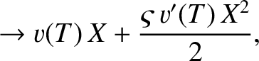

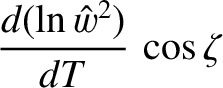
![$\displaystyle \rightarrow \xi\left[v(T) + \frac{1}{1+\tau}\left(1-\alpha_\theta\,\frac{\eta_i}{1+\eta_i}\right)+\varsigma\,v'(T)\,X\right],$](img3522.png)


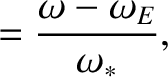

![$\displaystyle = -\frac{\hat{w}}{2\,\omega_\ast}\left[r\,\frac{d\omega_E}{dr}\right]_{r_{s-}}^{r_{s+}},$](img2724.png)