Asymptotic Matching

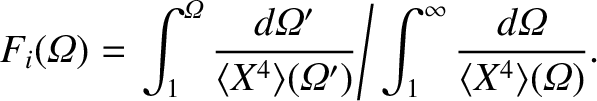
Now that we have found the solution of our rescaled, reduced, drift-MHD equations in the immediate vicinity of the magnetic island chain, it is necessary to asymptotically match this solution to the solution in the outer region. Given that $\hat{\mit\Psi}_s$ is real, it follows from Equations (3.72), (3.73), (3.183), (3.184), and (8.9) that

$${\rm Re}\!\left(\frac{{\mit\Delta}\hat{\mit\Psi}_s}{\hat{\mit\Psi}_s}\right) = \frac{2\,r_s}{R_0\,B_z\,\hat{\mit\Psi}_s}\int_{r_{s-}}^{r_{s+}}... ...}\oint \frac{\partial^2\psi}{\partial X^2}\,\cos\zeta\,\frac{d\zeta}{2\pi}\,dX,$$ (8.91)

$${\rm Im}\!\left(\frac{{\mit\Delta}\hat{\mit\Psi}_s}{\hat{\mit\Psi}_s}\right) = -\frac{2\,r_s}{R_0\,B_z\,\hat{\mit\Psi}_s}\int_{r_{s-}}^{r_{s+}... ...}\oint \frac{\partial^2\psi}{\partial X^2}\,\sin\zeta\,\frac{d\zeta}{2\pi}\,dX.$$ (8.92)

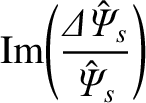
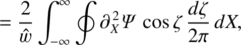
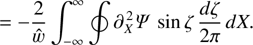
Making use of Equations (8.1) and (8.11), we obtain

$${\rm Re}\!\left(\frac{{\mit\Delta}\hat{\mit\Psi}_s}{\hat{\mit\Psi}_s}\right) =\frac{2}{\hat{w}}\int_{-\infty}^{\infty}\oint \partial_X^{\,2}{\mit\Psi}\,\cos\zeta\,\frac{d\zeta}{2\pi}\,dX,$$ (8.93)

$${\rm Im}\!\left(\frac{{\mit\Delta}\hat{\mit\Psi}_s}{\hat{\mit\Psi}_s}\right) =-\frac{2}{\hat{w}}\int_{-\infty}^{\infty}\oint \partial_X^{\,2}{\mit\Psi}\,\sin\zeta\,\frac{d\zeta}{2\pi}\,dX.$$ (8.94)

However, according to Equations (8.20) and (8.53),

$$\partial_X^{\,2}{\mit\Psi} = 1 + \epsilon_\beta\,\epsilon_c\,{\cal J}_0 + \epsilon\,\epsilon_\beta\,\epsilon_c\,{\cal J}_1.$$ (8.95)

Moreover, it is clear from Equations (8.80) and (8.85) that ${\cal J}_0$ has the symmetry of $\cos\zeta$, whereas ${\cal J}_1$ has the symmetry of $\sin\zeta$. Hence, we deduce that

$${\rm Re}\!\left(\frac{{\mit\Delta}\hat{\mit\Psi}_s}{\hat{\mit\Psi}_s}\right) =\frac{2\,\epsilon_\beta\,\epsilon_c}{\hat{w}}\int_{-\infty}^{\infty}\oint {\cal J}_0\,\cos\zeta\,\frac{d\zeta}{2\pi}\,dX,$$ (8.96)

$${\rm Im}\!\left(\frac{{\mit\Delta}\hat{\mit\Psi}_s}{\hat{\mit\Psi}_s}\right) =-\frac{2\,\epsilon_\beta\,\epsilon_c}{\hat{w}}\int_{-\infty}^{\infty}\oint \epsilon\,{\cal J}_1\,\sin\zeta\,\frac{d\zeta}{2\pi}\,dX.$$ (8.97)

The previous two equations can also be written

$${\rm Re}\!\left(\frac{{\mit\Delta}\hat{\mit\Psi}_s}{\hat{\mit\Psi}_s}\right) =\frac{4\,\epsilon_\beta\,\epsilon_c}{\hat{w}}\int_{-1}^\infty \langle {\cal J}_0\,\cos\zeta\rangle\,d{\mit\Omega},$$ (8.98)

$${\rm Im}\!\left(\frac{{\mit\Delta}\hat{\mit\Psi}_s}{\hat{\mit\Psi}_s}\right) =-\frac{4\,\epsilon_\beta\,\epsilon_c}{\hat{w}}\int_{-1}^\infty \... ...^\infty \langle X\,\epsilon\,\{{\cal J}_1,{\mit\Omega}\}\rangle\,d{\mit\Omega}.$$ (8.99)

Here, we have made use of the fact that ${\cal J}_0$ and ${\cal J}_1$ are both even functions of $X$, as well as the easily proved results $\partial(X,\zeta)/\partial({\mit\Omega},\zeta)= 1/X$ and $\{{\cal J}_1,{\mit\Omega}\} = -X\,(\partial{\cal J}_1/\partial\zeta)_{{\mit\Omega}}$.

Equations (8.85) and (8.99) can be combined to give [5]

$${\rm Im}\!\left(\frac{{\mit\Delta}\hat{\mit\Psi}_s}{\hat{\mit\Psi}_s}\right) =\frac{4\,\epsilon_\beta\,\epsilon_c\,\epsilon_\varphi}{\hat{w}}\... ...ga}(\vert X\vert^3\,\partial_{\mit\Omega}Y_i)\right]\right\rangle d{\mit\Omega}$$

$$=\frac{4\,\epsilon_\beta\,\epsilon_c\,\epsilon_\varphi}{\hat{w}}\... ...i + \langle \vert X\vert^5\rangle\,d_{\mit\Omega}^{\,2} Y_i\right)d{\mit\Omega}$$

$$= \frac{4\,\epsilon_\beta\,\epsilon_c\,\epsilon_\varphi}{\hat{w}}... ...it\Omega} Y_i + \langle \vert X\vert^5\rangle\,d_{\mit\Omega}^{\,2} Y_i\right),$$ (8.100)

where use has been made of the facts that $Y_i$ is zero inside the island separatrix, $Y_i$ is continuous across the separatrix, and $\partial_{\mit\Omega} X^n = n\,X^{n-2}$. Combining the previous equation with Equation (8.87), we obtain [5]

$${\rm Im}\!\left(\frac{{\mit\Delta}\hat{\mit\Psi}_s}{\hat{\mit\Psi... ...\right) =- \frac{4\,\epsilon_\beta\,\epsilon_c\,\epsilon_\varphi\,v'}{\hat{w}}.$$ (8.101)

The previous equation yields

$$\left[r\,\frac{d\omega_E}{dr}\right]_{r_{s-}}^{r_{s+}} = \left(\f... ...t){\rm Im}\!\left(\frac{{\mit\Delta}\hat{\mit\Psi}_s}{\hat{\mit\Psi}_s}\right),$$ (8.102)

where use has been made of Equations (8.23), (8.25), (8.27), and (8.46), as well as

$$\frac{L_p}{L_s} = \frac{c_\beta}{\omega_\ast\,\tau_H}\,\frac{d_\beta}{r_s}.$$ (8.103)

Here, $\tau _H$ is the hydromagnetic time [see Equation (5.43)]. Equation (8.102) can also be obtained by integrating Equation (3.165) across the rational surface, making use of Equation (3.140), as well as the identification

$$\left[r\,\frac{d\omega_E}{dr}\right]_{r_{s-}}^{r_{s+}} = m\left[r\,\frac{\partial{\mit\Delta\Omega}_\theta}{\partial r}\right]_{r_{s-}}^{r_{s+}}.$$ (8.104)

The previous identification merely states that the discontinuity in the MHD fluid velocity gradient that develops in the outer region at the rational surface is mirrored by an equal discontinuity in the ion fluid velocity gradient (because the discontinuity is ultimately due to a discontinuity in the E-cross-B velocity gradient, and there is no discontinuity in the diamagnetic velocity gradient).

Equations (8.80) and (8.98) can be combined to give

$${\rm Re}\!\left(\frac{{\mit\Delta}\hat{\mit\Psi}_s}{\hat{\mit\Psi}_s}\right) = \frac{4}{\epsilon_R\,\hat{w}}\,\frac{d(\ln \hat{w}^2)}{dT}\int_... ...mega}(M\,Y_i)\left\langle\widetilde{X^2}\,\cos\zeta\right\rangle d{\mit\Omega}.$$ (8.105)

Making use of Equations (8.76), (8.83), and (8.87), the previous equation yields

$${\rm Re}\!\left(\frac{{\mit\Delta}\hat{\mit\Psi}_s}{\hat{\mit\Psi}_s}\right) =\frac{4}{\epsilon_R\,\hat{w}}\,\frac{d(\ln \hat{w}^2)}{dT}\int_{... ...rangle}\right)\left\langle\widetilde{X^2}\,\cos\zeta\right\rangle d{\mit\Omega}$$

$$\phantom{=}+ \frac{2\,\epsilon_\beta\,\epsilon_c\,v'^{\,2}}{\hat{... ...^{\,2}\right)\left\langle\widetilde{X^2}\,\cos\zeta\right\rangle d{\mit\Omega},$$ (8.106)

where

$$F_i({\mit\Omega})=\left.\int_1^{\mit\Omega}\frac{d{\mit\Omega}'}{... ...}')}\right/\int_1^\infty\frac{d{\mit\Omega}}{\langle X^4\rangle({\mit\Omega})}.$$ (8.107)

Finally, Equations (8.10), (8.23)–(8.27), (8.101), (8.103), and (8.106) give [6,12]

$${\rm Re}\!\left(\frac{{\mit\Delta}\hat{\mit\Psi}_s}{\hat{\mit\Psi}_s}\right) = I_1\,\tau_R\,\frac{d}{dt}\!\left(\frac{4\,w}{r_s}\right) - I_2\... ...^2 {\rm Im}\!\left(\frac{{\mit\Delta}\hat{\mit\Psi}_s}{\hat{\mit\Psi}_s}\right)$$

$$\phantom{=} -I_3\left(\frac{\tau_\varphi}{\tau_H}\right)^2 \left(... ...}\!\left(\frac{{\mit\Delta}\hat{\mit\Psi}_s}{\hat{\mit\Psi}_s}\right)\right]^2,$$ (8.108)

where

$$I_1 = 2\int_{-1}^\infty \frac{\langle \cos\zeta\rangle^2}{\langle 1\rangle}\,d{\mit\Omega},$$ (8.109)

$$I_2 = \frac{1}{4}\int_1^\infty d_{\mit\Omega}\!\left(\frac{F_i}{\lang... ...X^4\rangle - \frac{\langle X^2\rangle^2}{\langle 1\rangle}\right)d{\mit\Omega},$$ (8.110)

$$I_3 = \frac{1}{16}\int_1^\infty d_{\mit\Omega}\!\left(F_i^{\,2}\right... ...X^4\rangle - \frac{\langle X^2\rangle^2}{\langle 1\rangle}\right)d{\mit\Omega}.$$ (8.111)