Higher-Order Solution

In order to include the perpendicular transport term, we need to evaluate Equation (8.16) to third order in $\epsilon$. Doing so, we obtain

$$\frac{d(\ln \hat{w}^{\,2})}{dT}\,\cos\zeta = \{F_e, {\mit\Omega}\} + \epsilon_\beta\,\epsilon_c\,\epsilon_R\,{\cal J}_0,$$ (8.77)

where

$$F_e({\mit\Omega},\zeta,T)= \epsilon^2\,({\mit\Phi}_2+\epsilon\,{\... ...\cal N}_3) - \epsilon^2\,\varsigma\,Y_e\,({\mit\Psi}_2+\epsilon\,{\mit\Psi}_3),$$ (8.78)

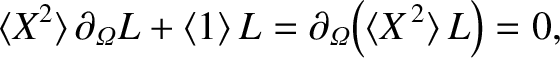
and use has been made of Equations (8.49)–(8.53), (8.57), (8.58), (8.61), (8.62), and (8.75). The flux-surface average of Equation (8.77) yields

$$\overline{\cal J}_0({\mit\Omega},T) = \frac{1}{\epsilon_\beta\,\e... ...frac{d(\ln \hat{w}^{2})}{dT}\,\frac{\langle\cos\zeta\rangle}{\langle 1\rangle},$$ (8.79)

where use has been made of Equations (8.68), (8.70), and (8.71). Hence, we can write

$${\cal J}_0({\mit\Omega},\zeta,T)= \frac{1}{\epsilon_\beta\,\epsil... ...angle} +\frac{1}{2}\,\partial_{\mit\Omega}\!\left(M\,Y_i\right)\widetilde{X^2},$$ (8.80)

where use has been made of Equation (8.76). The first term on the right-hand side of the previous equation represents the parallel current driven inductively when the reconnected flux at the rational surface varies in time. The second term on the right-hand side of the previous equation represents the parallel return current driven by the perpendicular polarization current associated with the acceleration of the ion fluid around the magnetic separatrix of the island chain [10,11]. In fact, it is easily seen that if the ion fluid could pass freely through the separatrix (i.e., ${\mit\Phi}_0\propto X$ and ${\cal N}_0\propto X$) then the polarization term would be zero.

In order to include the perpendicular transport term, we need to evaluate Equation (8.17) to first order in $\epsilon$. Doing so, we obtain

$$0= \epsilon\,\{{\cal V}_1, {\mit\Omega}\} + \epsilon^2\,\epsilon_... ...\Omega}\right\}+ \epsilon_\perp\,\varsigma\,(X^2\,\partial_{\mit\Omega} L + L),$$ (8.81)

where use has been made of Equations (8.49)–(8.53), (8.55), (8.57), and (8.58). The flux-surface average of the previous equation yields

$$\langle X^2\rangle\,\partial_{\mit\Omega} L +\langle 1\rangle\,L = \partial_{\mit\Omega}\!\left(\langle X^{\,2}\rangle\,L\right) = 0,$$ (8.82)

where use has been made of Equation (8.68). Here, we have made use of the easily proved result that $d_{\mit\Omega}\langle X^n\rangle = (n-1)\,\langle X^{n-2}\rangle$, where $d_{\mit\Omega}\equiv d/d{\mit\Omega}$. We can solve the previous equation, subject to the boundary condition (8.59), to give

$$L({\mit\Omega},T)= L({\mit\Omega})=\left\{ \begin{array}{llr}... ...5ex] 1/\langle X^2\rangle&~~&{\mit\Omega}>1 \end{array}\right..$$ (8.83)

Here, we have taken into account the previously mentioned fact that $L=0$ within the island separatrix.

Note that $L({\mit\Omega})$ is discontinuous across the island separatrix, which implies that the pressure gradient—and, hence, the diamagnetic velocity—is also discontinuous across the separatrix. Of course, there is not a real discontinuity. In fact, we would expect the discontinuity to be resolved in a layer on the separatrix whose width is obtained by balancing the parallel and perpendicular energy transport terms in Equation (8.17) [3]. In other words, we expect the layer thickness to correspond to the island width at which $\epsilon_\parallel\,\epsilon_\perp\sim 1$. Hence, according to Equations (8.28) and (8.29), the characteristic layer thickness is $4\,w_d$, where

$$w_d = \left(\frac{w_\parallel\,w_\perp^2}{4}\right)^{1/3},$$ (8.84)

and $w_\parallel$ and $w_\perp$ are specified in Equations (8.33) and (8.34), respectively. (The factor of 4 ensures that $W_d=4\,w_d$ has the same value as the standard critical island width, $W_c$, defined in Reference [3].) As is clear from Table 8.1, $w_d$ is of order half a centimeter in a tokamak fusion reactor.

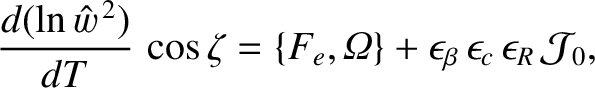
In order to include the perpendicular transport term, we need to evaluate Equation (8.18) to first order in $\epsilon$. Doing so, we obtain

$$0 =\epsilon\,\{{\cal J}_1,{\mit\Omega}\} +\epsilon_\varphi\,\vars... ...left[\partial_{\mit\Omega}\!\left(X^3\,\partial_{\mit\Omega} Y_i\right)\right].$$ (8.85)

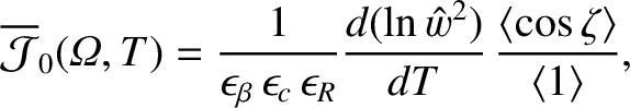
where use has been made of Equations (8.49)–(8.53), (8.55), (8.57), (8.58), (8.61), (8.62), and (8.76). The flux-surface average of the previous equation yields

$$\partial_{\mit\Omega}^{\,2}\!\left(\langle X^4\rangle\,d_{\mit\Omega} Y_i\right)= 0.$$ (8.86)

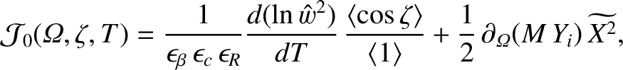
We can solve the previous equation, subject to the boundary conditions (8.59) and (8.63), to give

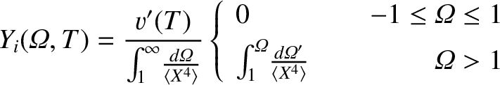$$Y_i({\mit\Omega},T)=\frac{v'(T)}{\int_1^\infty \!\frac{d{\mit... ...ega}'}{\langle X^4\rangle}&~~&{\mit\Omega}>1 \end{array}\right.$$ (8.87)

[5]. Here, we have rejected, as unphysical, the solution that blows up as ${\mit\Omega}^{\,1/2}$ as ${\mit\Omega}\rightarrow\infty$. We have also made use of the fact that $Y_i=0$ within the magnetic separatrix of the island chain. Finally, we have demanded that the ion fluid velocity—and, hence, the function $Y_i({\mit\Omega})$—be continuous across the separatrix, because the ion fluid possesses finite perpendicular viscosity. Note, however, that the discontinuity in the function $L({\mit\Omega})$ across the island separatrix [see Equation (8.83)] implies that the electron and MHD fluid velocities are discontinuous across the separatrix. (See Section 8.7.) As previously mentioned, these discontinuities are resolved in a layer of characteristic thickness $4\,w_d$ on the separatrix.

In order to include the perpendicular transport term, we need to evaluate Equation (8.19) to second order in $\epsilon$. Doing so, we obtain

$$0=\epsilon\left\{-\epsilon_c\,\varsigma\,M\,{\cal V}_1-\epsilon\,... ...ial_{\mit\Omega}^2 {\cal V}_{(0)} + \partial_{\mit\Omega}{\cal V}_{(0)}\right),$$ (8.88)

where use has been made of Equations (8.49)–(8.53) (8.55), (8.57), (8.58), (8.61), (8.62), and (8.65). The flux-surface average of the previous equation yields

$$\langle X^2\rangle\,\partial_{\mit\Omega}^2 {\cal V}_{(0)} +\lang... ...ga}\!\left( \langle X^2\rangle\,\partial_{\mit\Omega} {\cal V}_{(0)}\right)= 0.$$ (8.89)

The previous equation can be solved, subject to the boundary condition (8.43), to give

$${\cal V}_{(0)}({\mit\Omega}, T) = 0.$$ (8.90)

Hence, we conclude that the lowest-order ion parallel flow is unaffected by the presence of the island chain.