Rescaled Reduced Drift-MHD Model

Let

$$X = \frac{\hat{x}}{\hat{w}},$$ (8.9)

$$T = \omega_\ast\,t= \hat{\omega}_\ast\,\hat{t},$$ (8.10)

where $\omega _\ast$ is the diamagnetic frequency at the rational surface [see Equation (5.47)], and $\hat{\omega}_\ast = \omega_\ast/(V_A/r_s)$. It follows that $\vert X\vert\sim {\cal O}(1)$ in the immediate vicinity of the island chain.

It is helpful to define the rescaled fields ${\mit\Psi}(X,\zeta,T)$, ${\cal N}(X,\zeta,T)$, ${\mit\Phi}(X,\zeta,T)$, ${\cal V}(X,\zeta,T)$, and ${\cal J}(X,\zeta,T)$, where

$$\psi = \left(\frac{\hat{w}^{\,2}}{\hat{L}_s}\right){\mit\Psi},$$ (8.11)

$$N = \left(\frac{\hat{\omega}_\ast\,\hat{w}}{m}\right){\cal N},$$ (8.12)

$$\phi =\left(\frac{\hat{\omega}_\ast\,\hat{w}}{m}\right){\mit\Phi},$$ (8.13)

$$V = \tilde{V}_\parallel + \left(\frac{\hat{L}_s\,\hat{\omega}_\ast^{\,2}}{m^2\,c_\beta^{\,2}}\right){\cal V},$$ (8.14)

$$J =-\left(\frac{2}{s_s}-1\right)\frac{1}{\hat{L}_s} + \left(\frac{\hat{L}_s\,\hat{\omega}_\ast^{\,2}}{m^2\,\hat{w}^{\,2}}\right){\cal J}.$$ (8.15)

Here, $c_\beta$ a dimensionless measure of the plasma pressure at the rational surface [see Equation (4.65)].

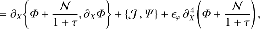
The reduced drift-MHD model specified in Section 5.2 rescales to give

$$\frac{d(\ln \hat{w}^2)}{dT}\,\cos\zeta = \left\{{\mit\Phi}-\left(\frac{\tau}{1+\tau}\right)\,{\cal N}, {\mit\Psi}\right\} + \epsilon_\beta\,\epsilon_c\,\epsilon_R\,{\cal J},$$ (8.16)

$$\frac{\partial {\cal N}}{\partial T} = \{{\mit\Phi}, {\cal N}\} + \{{\cal V},{\mit\Psi}\} + \epsilon_c... ...\{{\cal N},{\mit\Psi}\}, {\mit\Psi}\}+\epsilon_\perp\,\partial_X^{\,2}{\cal N},$$ (8.17)

$$\frac{\partial(\partial_X^{\,2}\,{\mit\Phi})}{\partial T} = \partial_X\!\left\{{\mit\Phi} + \frac{{\cal N}}{1+\tau},\partia... ...on_\varphi \,\partial_X^{\,4}\left({\mit\Phi} + \frac{{\cal N}}{1+\tau}\right),$$ (8.18)

$$\epsilon_c\,\frac{\partial {\cal V}}{\partial T} = \epsilon_c\,\{{\mit\Phi},{\cal V}\}+\{{\cal N}, {\mit\Psi}\} + \epsilon_c\,\epsilon_\varphi\,\partial_X^{\,2} {\cal V},$$ (8.19)

$$\partial_X^{\,2}{\mit\Psi} = 1+ \epsilon_\beta\,\epsilon_c\,{\cal J}.$$ (8.20)

Here, $\partial_X\equiv \partial/\partial X$,

$$\{A,B\} \equiv \frac{\partial A}{\partial X}\,\frac{\partial B}{\partial\zeta} - \frac{\partial A}{\partial \zeta}\,\frac{\partial B}{\partial X},$$ (8.21)

and we have set

$$\hat{E}_\parallel = \left(\frac{2}{s_s}-1\right)\frac{\hat{\eta}_\parallel}{\hat{L}_s}$$ (8.22)

[see Equation (5.32)], where $\hat{\eta}_\parallel$ is the normalized parallel plasma resistivity at the rational surface [see Equation (5.14)]. Furthermore,

$$\epsilon_\beta = c_\beta^{\,2},$$ (8.23)

$$\epsilon_p = \left(\frac{L_p}{L_s}\right)^2,$$ (8.24)

$$\epsilon_c = \left(\frac{L_s}{L_p}\right)^2\left(\frac{d_\beta}{w}\right)^2= \left(\frac{w_c}{w}\right)^2,$$ (8.25)

$$\epsilon_R = \frac{r_s^{\,2}}{\omega_\ast\,\tau_R\,w^2}=\left(\frac{w_R}{w}\right)^2,$$ (8.26)

$$\epsilon_\varphi = \frac{r_s^{\,2}}{\omega_\ast\,\tau_\varphi\,w^2}=\left(\frac{w_\varphi}{w}\right)^2,$$ (8.27)

$$\epsilon_\perp = \frac{r_s^{\,2}}{\omega_\ast\,\tau_\perp\,w^2}= \left(\frac{w_\perp}{w}\right)^2,$$ (8.28)

$$\epsilon_\parallel = \frac{\omega_\ast\,\tau_\parallel'\,r_s}{(\epsilon_s\,s_s\,n)^2\,w}=\frac{w_\parallel}{w},$$ (8.29)

where

$$w_c = \frac{L_s\,d_\beta}{L_p},$$ (8.30)

$$w_R = \frac{r_s}{\sqrt{\omega_\ast\,\tau_R}},$$ (8.31)

$$w_\varphi = \frac{r_s}{\sqrt{\omega_\ast\,\tau_\varphi}},$$ (8.32)

$$w_\perp = \frac{r_s}{\sqrt{\omega_\ast\,\tau_\perp}},$$ (8.33)

$$w_\parallel = \frac{\omega_\ast\,\tau_\parallel'\,r_s}{(\epsilon_s\,s_s\,n)^2}.$$ (8.34)

Here, $d_\beta= c_\beta\,d_i$ is the ion sound radius, $\tau _R$ the resistive diffusion time [see Equation (5.49)], $\tau _\varphi$ the toroidal momentum confinement time [see Equation (5.50)], and $\tau _\perp$ the energy confinement time [see Equation (5.52)]. All of these quantities are evaluated at the rational surface. Moreover,

$$L_p=\frac{5}{3}\,(1-c_\beta^2) \left[-\left(\frac{d\ln p}{dr}\right)_{r_s}\right]^{-1}$$ (8.35)

is the effective pressure gradient scale-length at the rational surface, and $\epsilon_s=r_s/R_0$. Finally,

$$\tau_\parallel' = r_s^{\,2}\left/\left\{\frac{2}{3}\,(1-c_\beta^2... ...(\frac{\eta_i}{1+\eta_i}\right)\chi_{\parallel\,i}'(r_s)\right]\right\}\right.,$$ (8.36)

where

$$\chi_{\parallel\,e}' = \frac{v_{t\,e}\,L_s}{2\,\pi^{1/2}\,m},$$ (8.37)

$$\chi_{\parallel\,i}' = \frac{v_{t\,i}\,L_s}{2\,\pi^{1/2}\,m}.$$ (8.38)

Here, $v_{t\,e}$ and $v_{t\,i}$ are the electron and ion thermal velocities, respectively [see Equation (2.17)]. Note that the parallel electron and ion energy diffusivities have been estimated from Equations (2.319) and (2.320), respectively, on the assumption that $k_\parallel \simeq 2\,(m/L_s)\,\hat{w}$, which is the typical parallel wavenumber of the tearing perturbation at the edge of a magnetic island chain of reduced width $w$. Note that in writing Equation (8.18) we have made use of the easily proved identity

$$\{{\mit\Phi},\partial_X^{\,2}{\mit\Phi}\}-\frac{1}{2\,(1+\tau)}\l... ...al_X\!\left\{{\mit\Phi} + \frac{{\cal N}}{1+\tau},\partial_X{\mit\Phi}\right\}.$$ (8.39)

Equations (8.16)–(8.20) must be solved subject to the boundary conditions [see Equations (8.2)–(8.6) and (8.11)–(8.15)]

$${\mit\Psi}(X,\zeta,T) \rightarrow \frac{X^{2}}{2} + \cos\zeta,$$ (8.40)

$${\cal N}(X,\zeta,T) \rightarrow X,$$ (8.41)

$${\mit\Phi}(X,\zeta,T) \rightarrow v(T)\,X +\frac{\varsigma\,v'(T)\,X^{2}}{2},$$ (8.42)

$${\cal V}(X,\zeta,T) \rightarrow 0,$$ (8.43)

$${\cal J}(X,\zeta,T) \rightarrow 0,$$ (8.44)

as $\vert X\vert\rightarrow\infty$. Here,

$$v(T) = \frac{\omega-\omega_E(r_s)}{\omega_\ast},$$ (8.45)

$$v'(T) = -\frac{\hat{w}}{2\,\omega_\ast}\left[r\,\frac{d\omega_E}{dr}\right]_{r_{s-}}^{r_{s+}},$$ (8.46)

where $\omega_E(r)= (m/r)\,V_E(r)$ is the E-cross-B frequency profile. Note that ${\mit\Psi}$, ${\cal N}$, ${\mit\Phi}$, ${\cal V}$, and ${\cal J}$ are all ${\cal O}(1)$ quantities in the inner region. Note, further, that the boundary conditions (8.40)–(8.44), as well as the symmetry of the rescaled, reduced, drift-MHD equations, (8.16)–(8.20), ensure that ${\mit\Psi}$, ${\cal V}$, and ${\cal J}$ are even functions of $X$, whereas ${\cal N}$ and ${\mit\Phi}$ are odd functions.