Next: Magnetic Field-Line Curvature Up: Nonlinear Neoclassical Resonant Response Previous: Neoclassical Drift-MHD Equations Contents
 , and the collisionless ion skin-depth,
  , are defined in Equations (4.23) and
(4.24), respectively. Let
, are defined in Equations (4.23) and
(4.24), respectively. Let  be a typical variational lengthscale in the inner region. It is convenient to adopt the
following normalization scheme that renders all quantities in the neoclassical drift-MHD fluid equations dimensionless:
be a typical variational lengthscale in the inner region. It is convenient to adopt the
following normalization scheme that renders all quantities in the neoclassical drift-MHD fluid equations dimensionless:
 ,
,
 ,
,
 ,
,
 ,
,
 ,
,
 ,
,
 ,
,
 ,
,
 ,
,
 ,
,
 ,
,
 ,
,
 ,
,
 ,
,
 ,
,
 ,
,
 .
Here,
.
Here,
 is the ion parallel fluid velocity [see Equation (2.321)].
Equations (11.1)–(11.3) yield the following set of
normalized neoclassical drift-MHD fluid equations:
where
Finally, Maxwell's equations yield
is the ion parallel fluid velocity [see Equation (2.321)].
Equations (11.1)–(11.3) yield the following set of
normalized neoclassical drift-MHD fluid equations:
where
Finally, Maxwell's equations yield
As before (see Section 4.4), all quantities in the inner region are assumed to be functions of  ,
,
 , and
, and  only. Here,
  and
and  are the poloidal and toroidal angles, respectively, whereas
  and
and  are the
poloidal and toroidal mode numbers, respectively, of the tearing mode. (See Sections 3.2 and 3.3.)
We can write
are the
poloidal and toroidal mode numbers, respectively, of the tearing mode. (See Sections 3.2 and 3.3.)
We can write
 |
 |
(11.28) |
 |
 |
(11.29) |
 |
 |
(11.30) |
 |
 |
(11.31) |
 |
 |
(11.32) |
 |
 |
(11.33) |
 |
 |
(11.34) |
 is defined in Equation (4.37),
 is the (normalized) constant inductive component of the parallel electric field that maintains the equilibrium parallel current density in the inner region against ohmic decay, and
 . The superscript
  indicates a quantity that is
first order in our ordering scheme. Zeroth order terms are left without superscripts, whereas second order terms are given the superscript (2).
indicates a quantity that is
first order in our ordering scheme. Zeroth order terms are left without superscripts, whereas second order terms are given the superscript (2).
Evaluating the normalized neoclassical drift-MHD fluid equations, (11.16)–(11.18), up to second order, we obtain
where is defined in Equation (4.49),
![$[A,B]\equiv \hat{\nabla}A\times \hat{\nabla}B\cdot{\bf n}$](img1984.png) , and
, and
 |
 |
(11.38) |
 |
 |
(11.39) |
To first order, Equations (11.35) and (11.36) again give the equilibrium force balance constraint
(See Section 4.4.) The scalar product of Equation (11.35) with yields
The
scalar product of Equation (11.36) with gives
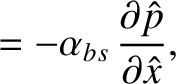
The scalar product of the curl of Equation (11.35) with yields
Finally, the scalar product of the curl of Equation (11.36) with gives
![$\displaystyle \hat{\nabla}^2{\mit\Upsilon}^{(2)} = 2\left[\delta p^{(1)}, \phi^{(1)}\right] +\hat{d}_i\left[J^{(1)}, \psi^{(1)}\right].$](img1924.png) |
(11.44) |
 is defined in Equations (4.65) and (4.66).
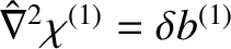
Our final reduced neoclassical drift-MHD model takes the form [7,8,10]
where Here, we have suppressed the ordering superscripts. If we compare Equations (11.46)–(11.51), to our previous reduced non-neoclassical drift-MHD equations, (4.67)–(4.74), then we can see that the former set of equations contain many additional terms. The additional term involving the parameter in Equation (11.46)
is due to the bootstrap current. The additional terms involving the parameters
in Equation (11.46)
is due to the bootstrap current. The additional terms involving the parameters
 and
and
 in
Equation (11.47) are due to neoclassical parallel momentum and heat fluxes.
Finally, the additional terms involving the parameter
in
Equation (11.47) are due to neoclassical parallel momentum and heat fluxes.
Finally, the additional terms involving the parameter
 in Equations (11.48)
and (11.49) are due to neoclassical poloidal flow damping.
in Equations (11.48)
and (11.49) are due to neoclassical poloidal flow damping.

![$\displaystyle \left. + (\hat{\nabla}\cdot\hat{\bf V}_E)\,\hat{\bf V}_\ast- (\ha...
...E\times\hat{\bf V}_\ast)\right]
+\hat{\nabla}\hat{p} -\hat{\bf j}\times {\bf b}$](img3409.png)


![$\displaystyle \frac{3}{2}\,\frac{\partial\hat{p}}{\partial\hat{t}}+\frac{3}{2}\...
...hat{j}_{bs}+\frac{\hat{E}_\parallel}{\hat{\eta}_\parallel}\right){\bf b}\right]$](img3412.png)


![$\displaystyle \hat{\nabla}\left(\delta p^{(1)}+ \delta b^{(1)}\right)+\left(\fr...
...l^{(1)},\phi^{(1)}\right] +\left[\psi^{(1)},\delta b^{(1)}\right]\right){\bf n}$](img3425.png)


![$\displaystyle \frac{3}{2}\,\frac{\partial^{(1)}\delta p^{(1)}}{\partial\hat{t}}...
...{V}_\parallel^{(1)},\psi^{(1)}\right]+\hat{\nabla}^2{\mit\Upsilon}^{(2)}\right)$](img3431.png)
![$\displaystyle +\frac{5}{2}\,\lambda\,\hat{p}_0\,\hat{d}_i\,[\delta p^{(1)},\del...
...{(1)}}\left[\frac{\partial^{(1)}\psi^{(1)}}{\partial \hat{t}},\psi^{(1)}\right]$](img3432.png)
![$\displaystyle -\hat{\chi}_\parallel^{(-1)}\left[\left[\delta p^{(1)},\psi^{(1)}\right],\psi^{(1)}\right]-\hat{\chi}_\perp^{(1)}\,\hat{\nabla}^2\delta p^{(1)}=0,$](img3433.png)
![$\displaystyle =\left[\phi^{(1)},\hat{V}_\parallel^{(1)}\right] -\left[\delta p^{(1)},\psi^{(1)}\right]$](img3441.png)
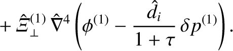
![$\displaystyle \phantom{=}-\hat{\mit\Xi}_\theta^{(1)}\,\frac{\epsilon^{(1)}}{q_s...
...ght]
\right) +\hat{\mit\Xi}_\perp^{(1)}\,\hat{\nabla}^2\hat{V}_\parallel^{(1)}.$](img3442.png)

![$\displaystyle = \left[\phi^{(1)}, \hat{\nabla}^2\phi^{(1)}\right]+\frac{\hat{d}...
...ta p ^{(1)}\right]
+\left[\hat{\nabla}^2\delta p^{(1)},\phi^{(1)}\right]\right)$](img3445.png)
![$\displaystyle \phantom{=} +\left[J^{(1)},\psi^{(1)}\right]+ \hat{\mit\Xi}_\thet...
...ft(1-\alpha_\theta\,\frac{\eta_i}{1+\eta_i}\right)\delta p^{(1)}\right]
\right)$](img3446.png)
![$\displaystyle = \left[\phi^{(1)},\delta p^{(1)}\right]
-c_\beta^{\,2}\left[\hat...
...t[\alpha_{nc}\,\frac{\partial\delta p^{(1)}}{\partial\hat{x}},\psi^{(1)}\right]$](img3448.png)


![$\displaystyle = \left[\phi,\psi\right] +\hat{d}_i\,\frac{\tau}{1+\tau}\left[\de...
...lpha_{bs}\,\frac{\partial\delta p}{\partial\hat{x}}\right) + \hat{E}_\parallel,$](img3450.png)

![$\displaystyle = \left[\phi,\delta p\right]
-c_\beta^{\,2}\left[\hat{V}_{\parall...
...el}}{\hat{\eta}_{\parallel}}\,\frac{\partial\psi}{\partial\hat{t}}, \psi\right]$](img3452.png)
![$\displaystyle \phantom{=}
+\frac{2}{3}\,(1-c_\beta^2)\,\hat{\chi}_\parallel\lef...
...ht] + \frac{2}{3}\,(1-c_\beta^2)\,\hat{\chi}_\perp\,\hat{\nabla}^{\,2}\delta p,$](img3453.png)

![$\displaystyle = \left[\phi, U\right]+\frac{\hat{d}_i}{2\,(1+\tau)}
\left(\hat{\...
...right]+\left[U,\delta p\right]
+\left[\hat{\nabla}^2\delta p,\phi\right]\right)$](img3454.png)
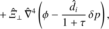
![$\displaystyle \phantom{=} +\left[J,\psi\right]+ \hat{\mit\Xi}_\theta\,\frac{\pa...
...au}\left(1-\alpha_\theta\,\frac{\eta_i}{1+\eta_i}\right)\delta p\right]
\right)$](img3455.png)

![$\displaystyle =\left[\phi,\hat{V}_\parallel\right] -\left[\delta p,\psi\right]-...
...au}\left(1-\alpha_\theta\,\frac{\eta_i}{1+\eta_i}\right)\delta p\right]
\right)$](img3458.png)