Next: Reduced Neoclasssical Drift-MHD Model Up: Nonlinear Neoclassical Resonant Response Previous: Introduction Contents
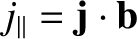
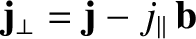
 ,
,  ,
,  ,
,  ,
,  , and
, and  that parameterize the equilibrium plasma density, pressure, and temperature, and
their gradients, at the rational surface. We also make the simplifying assumption that
perturbed electron and ion temperature profiles in the inner region are functions of the perturbed electron number density profile. Our neoclassical fluid equations, (2.370)–(2.374),
reduce to the following set of
neoclassical drift-MHD fluid equations:
Here, the E-cross-B, diamagnetic, MHD, and ion fluid velocities,
that parameterize the equilibrium plasma density, pressure, and temperature, and
their gradients, at the rational surface. We also make the simplifying assumption that
perturbed electron and ion temperature profiles in the inner region are functions of the perturbed electron number density profile. Our neoclassical fluid equations, (2.370)–(2.374),
reduce to the following set of
neoclassical drift-MHD fluid equations:
Here, the E-cross-B, diamagnetic, MHD, and ion fluid velocities,  ,
,
 ,
,  , and
, and  ,
respectively, are defined in Equations (4.10)–(4.13).
Moreover, the dimensionless parameter
,
respectively, are defined in Equations (4.10)–(4.13).
Moreover, the dimensionless parameter  , the ion perpendicular momentum diffusivity
 , the
parallel energy diffusivity
, the
parallel energy diffusivity
 , and the perpendicular energy diffusivity
 , are defined in Equations (4.16)–(4.19).
Finally,
Here,
, are defined in Equations (4.16)–(4.19).
Finally,
Here,  is a radial cylindrical coordinate,
 is a unit vector in the poloidal direction (see Section 3.2),
  is the minor radius of the rational surface,
 is the safety-factor at the rational surface [see Equation (3.2)],
 is the inverse aspect-ratio at the
rational surface [see Equation (3.18)], the ion neoclassical poloidal
flow-damping time
is the inverse aspect-ratio at the
rational surface [see Equation (3.18)], the ion neoclassical poloidal
flow-damping time
 is defined in Equation (2.332), the fraction of trapped particles
  is defined in Equation (2.202),
the dimensionless neoclassical parameters
is defined in Equation (2.202),
the dimensionless neoclassical parameters
 ,
,  ,
,  ,
,
 ,
,
 ,
,
 ,
,
 ,
,
 , and
, and
 are defined in Equations (2.209), (2.217), (2.218),
(2.243), (2.244), (2.247), (2.251), (2.347), and (2.348), respectively, and the
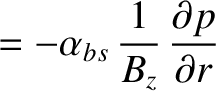
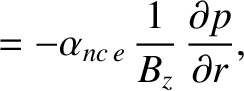
plasma perpendicular electrical conductivity
are defined in Equations (2.209), (2.217), (2.218),
(2.243), (2.244), (2.247), (2.251), (2.347), and (2.348), respectively, and the
plasma perpendicular electrical conductivity
 is defined in Equation (2.41). As before,
  is the magnitude of the electron charge,
  the
ion mass, the equilibrium electron number density at the rational surface, the equilibrium total
plasma pressure at the rational surface,
the
ion mass, the equilibrium electron number density at the rational surface, the equilibrium total
plasma pressure at the rational surface,  the electric field-strength,
  the magnetic field-strength,
 the current density,
  the total plasma pressure, and
 . Finally,
 ,
,
 , and
, and
 .
.
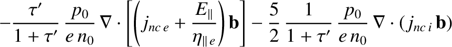
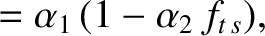
If we compare Equation (11.1) with its non-neoclassical concomitant, (4.7), then we can see that the former equation contains an
additional term that is due to the action of ion neoclassical poloidal flow damping. The term in question involves
 , which is the ion neoclassical poloidal
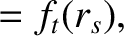
flow-damping time at the rational surface. If we compare Equation (11.2) with its non-neoclassical concomitant, (4.8), then
we can see that the former equation contains an additional term that is due to the action of the bootstrap current. The term in question involves
, which is the ion neoclassical poloidal
flow-damping time at the rational surface. If we compare Equation (11.2) with its non-neoclassical concomitant, (4.8), then
we can see that the former equation contains an additional term that is due to the action of the bootstrap current. The term in question involves
 , which is the parallel bootstrap current density at the rational surface. Finally, if we compare Equation (11.3)
with its non-neoclassical concomitant, (4.9), then we can see that the former equation contains many additional terms that are due to
neoclassical parallel momentum and heats flows.
, which is the parallel bootstrap current density at the rational surface. Finally, if we compare Equation (11.3)
with its non-neoclassical concomitant, (4.9), then we can see that the former equation contains many additional terms that are due to
neoclassical parallel momentum and heats flows.
![$\displaystyle m_i\,n_0\left[\frac{\partial {\bf V}}{\partial t} + ({\bf V}\cdot...
...au}\,({\bf V}_\ast\cdot\nabla){\bf V}_E\right]+\nabla p - {\bf j}\times {\bf B}$](img3352.png)


![$\displaystyle \frac{3}{2}\,\frac{\partial p}{\partial t} +\frac{3}{2}\,{\bf V}\...
...cdot
\left[\left(j_{bs}+\frac{E_\parallel}{\eta_\parallel}\right){\bf b}\right]$](img3355.png)


![$\displaystyle = f_{t\,s}\,\frac{q_s}{\epsilon_s}\left[\beta_{11}\left(1-\alpha_...
...+\eta_i}\right)
-\beta_{12}\,\frac{\tau}{1+\tau}\frac{\eta_e}{1+\eta_e}\right],$](img3375.png)

![$\displaystyle = f_{t\,s}\,\frac{q_s}{\epsilon_s}\left[\epsilon_1\left(1-\alpha_...
...+\eta_i}\right)
-\epsilon_2\,\frac{\tau}{1+\tau}\frac{\eta_e}{1+\eta_e}\right],$](img3377.png)