Suppose that, at  , a solenoid of inductance
  , and resistance
  , is connected
across the terminals of a battery of voltage
, is connected
across the terminals of a battery of voltage  . The circuit equation is
 |
(2.358) |
[See Equation (2.326).]
The power output of the battery is  . [Every charge
  that goes around the circuit
falls through a potential difference
that goes around the circuit
falls through a potential difference  . In order to raise it back to
the starting potential, so that it can perform another circuit, the battery must do
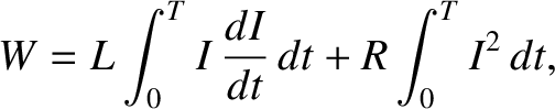
work . See Section 2.1.5. The work done per unit time (i.e., the power) is
. In order to raise it back to
the starting potential, so that it can perform another circuit, the battery must do
work . See Section 2.1.5. The work done per unit time (i.e., the power) is  , where
  is
the number of charges per unit time passing a given point on the circuit.
But,
is
the number of charges per unit time passing a given point on the circuit.
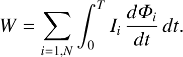
But,  , so the power output is .] Thus, the net work done by the battery in
raising the current in the circuit from zero at time to
, so the power output is .] Thus, the net work done by the battery in
raising the current in the circuit from zero at time to  at
time
at
time  is
is
 |
(2.359) |
Using the circuit equation (2.358), we obtain
 |
(2.360) |
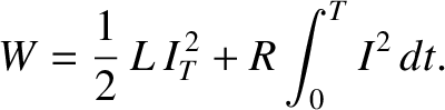
giving
 |
(2.361) |
The second term on the right-hand side of the previous equation represents the irreversible conversion of
electrical energy into heat energy by the resistor. (See Section 2.1.11.) The first term is the amount of
energy stored in the solenoid at time  . This energy can be recovered after the
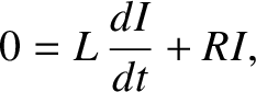
solenoid is disconnected from the battery. Suppose that the battery is disconnected
at time . The circuit equation is now
. This energy can be recovered after the
solenoid is disconnected from the battery. Suppose that the battery is disconnected
at time . The circuit equation is now
 |
(2.362) |
giving
![$\displaystyle I= I_T \exp \left[ - \frac{R}{L} \,(t-T)\right],$](img1834.png) |
(2.363) |
where we have made use of the initial condition
 .
Thus, the current
decays away exponentially. The energy stored in the solenoid is dissipated as
heat in the resistor. The total heat energy appearing in the resistor after the
battery is disconnected is
.
Thus, the current
decays away exponentially. The energy stored in the solenoid is dissipated as
heat in the resistor. The total heat energy appearing in the resistor after the
battery is disconnected is
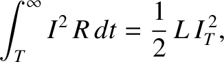 |
(2.364) |
where use has been made of Equation (2.363).
Thus, the heat energy appearing in the resistor is equal to the
energy stored in the solenoid. This energy is actually stored in the magnetic
field generated inside the solenoid.
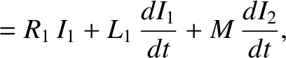
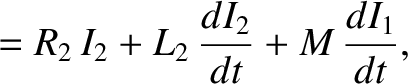
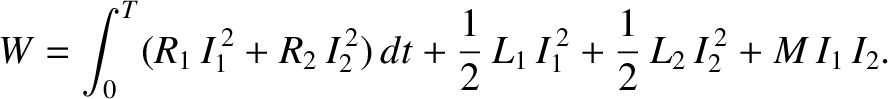
Consider, again, our circuit with two solenoids wound on top of one another. (See the previous section.) Suppose that
each solenoid is connected to its own battery. The circuit equations are thus
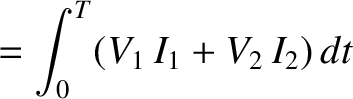
where  is the voltage of the battery in the first circuit, et cetera. The net work done by the two batteries in increasing the currents in the two circuits,
from zero at time 0, to
is the voltage of the battery in the first circuit, et cetera. The net work done by the two batteries in increasing the currents in the two circuits,
from zero at time 0, to  and
and  at time , respectively, is
Thus,
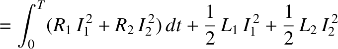
at time , respectively, is
Thus,
 |
(2.368) |
Clearly, the total magnetic energy stored in the two solenoids is
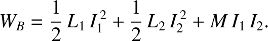 |
(2.369) |
Note that the mutual inductance term increases the stored magnetic energy if and
are of the same sign; that is, if the currents in the two solenoids flow
in the same direction, so that they generate magnetic fields that reinforce
one another. Conversely, the mutual inductance term decreases the stored
magnetic energy if and are of the opposite sign. However, the total
stored energy can never be negative, otherwise the coils
would constitute a power source (a negative stored energy is equivalent to
a positive generated energy). Thus,
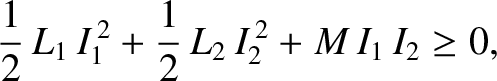 |
(2.370) |
which can be written
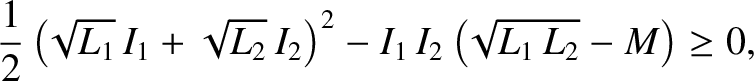 |
(2.371) |
assuming that
 . It follows that
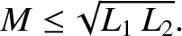 |
(2.372) |
The equality sign corresponds to the situation in which
all of the magnetic flux generated by one solenoid passes through the other. If some of
the flux misses then the inequality sign is appropriate.
In fact, the previous formula is valid
for any two inductively coupled circuits, and effectively sets an upper limit
on their mutual inductance.
We intimated previously that the energy stored in an solenoid is actually
stored in the surrounding magnetic field. Let us now obtain an
explicit formula for the energy stored in a magnetic field. Consider an ideal
cylindrical solenoid. The energy stored in the solenoid when a current  flows through it
is
flows through it
is
 |
(2.373) |
where is the self inductance. We know that
 |
(2.374) |
where  is the number of turns per unit length of the
solenoid,
is the number of turns per unit length of the
solenoid,  the radius, and
  the length. [See Equation (2.324).] The magnetic field inside the solenoid is approximately
uniform, with magnitude
the length. [See Equation (2.324).] The magnetic field inside the solenoid is approximately
uniform, with magnitude
 |
(2.375) |
and is approximately zero outside the solenoid. [See Equation (2.279).] Equation (2.373) can be rewritten
 |
(2.376) |
where
 is the volume of the solenoid. The previous formula strongly
suggests that a magnetic field possesses an energy density
is the volume of the solenoid. The previous formula strongly
suggests that a magnetic field possesses an energy density
 |
(2.377) |
Let us now examine a more general proof of the previous formula. Consider a system
of circuits (labeled  to ), each carrying a current
  .
The magnetic flux through the
.
The magnetic flux through the  th circuit is written [see Equation (2.315)]
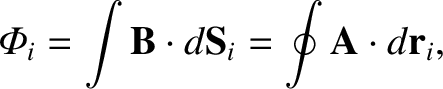 |
(2.378) |
where
 , and
, and
 and
and
 denote a
surface element and a line element of this circuit, respectively. The
back-emf induced in the th circuit follows from Faraday's law:
denote a
surface element and a line element of this circuit, respectively. The
back-emf induced in the th circuit follows from Faraday's law:
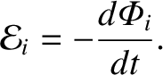 |
(2.379) |
[See Equation (2.284).]
The rate of work of the battery that maintains the current
in the th circuit
against this back-emf is
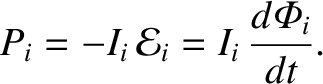 |
(2.380) |
Thus, the total work required
to raise the currents in the circuits from zero at time
0, to  at time , is
 |
(2.381) |
The previous expression for the work done is, of course, equivalent to the total
energy stored in the magnetic field surrounding the various circuits.
This energy is independent of the manner in which the currents
are set up.
Suppose, for the sake of simplicity, that the currents are ramped up linearly,
so that
 |
(2.382) |
The fluxes are proportional to the currents, so they must also ramp up linearly; that is,
 |
(2.383) |
It follows that
 |
(2.384) |
giving
 |
(2.385) |
So, if instantaneous currents flow in the circuits, which link
instantaneous fluxes
 , then the instantaneous stored energy is
 |
(2.386) |
Equations (2.378) and (2.386) imply that
 |
(2.387) |
It is convenient, at this stage, to replace our line currents by
current
distributions of
small, but finite, cross-sectional area.
Equation (2.387)
transforms to give
 |
(2.388) |
where is a volume that contains all of the circuits.
Note that for an element of the th circuit,
 and
and
 , where
  is the cross-sectional area of the
circuit.
Now,
is the cross-sectional area of the
circuit.
Now,
 [see Equation (2.271)], so
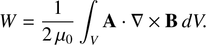 |
(2.389) |
However,
 |
(2.390) |
(see Section A.24),
which implies that
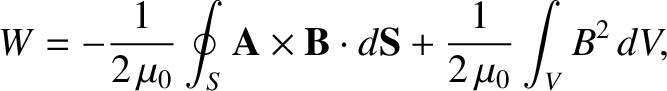
![$\displaystyle W = \frac{1}{2\,\mu_0} \int_V \left[- \nabla\cdot ({\bf A} \times{\bf B})
+{\bf B}\cdot \nabla \times {\bf A} \right] \,dV.$](img1880.png) |
(2.391) |
Using the divergence theorem (see Section A.20), and
, we obtain
 |
(2.392) |
where  is the bounding surface of some volume . Let us take this surface
to infinity. It is easily demonstrated that the magnetic field generated by a current
loop falls of like
is the bounding surface of some volume . Let us take this surface
to infinity. It is easily demonstrated that the magnetic field generated by a current
loop falls of like  at large distances. (See Section 2.2.7.) The vector potential
falls off like
at large distances. (See Section 2.2.7.) The vector potential
falls off like  . However, the area of surface only increases like
  .
It follows that the surface integral is negligible in the limit
.
It follows that the surface integral is negligible in the limit
 .
Thus, the previous expression reduces to
.
Thus, the previous expression reduces to
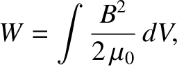 |
(2.393) |
where the integral is over all space.
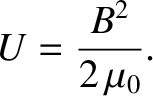
Because this expression is valid for any magnetic field whatsoever, we can safely conclude
that the energy density of a general magnetic field generated by a system of electrical circuits is given by
|
(2.394) |
Note, finally, that the fact that a magnetic field possesses an energy density demonstrates that it has a real physical
existence, and is not merely an aid to calculating the forces that current-carrying wires exert on one another.