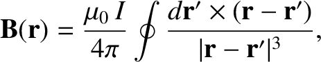
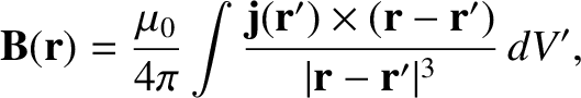
Biot-Savart Law
Consider a closed
electric circuit of general shape, fabricated from an idealized zero thickness wire, around which a current  flows. According to Biot-Savart law, which is named after Jean-Baptiste Biot and Félix Savart, and which can
be experimentally verified,
the magnetic field generated by such a circuit is
flows. According to Biot-Savart law, which is named after Jean-Baptiste Biot and Félix Savart, and which can
be experimentally verified,
the magnetic field generated by such a circuit is
 |
(2.226) |
where  is an element of the wire, whose displacement is
  ,
and the integral is taken around the whole circuit.
,
and the integral is taken around the whole circuit.
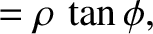
Figure 2.20:
A Biot-Savart law calculation.
|
|
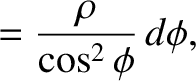
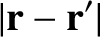
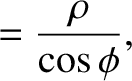
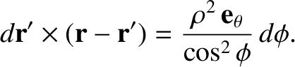
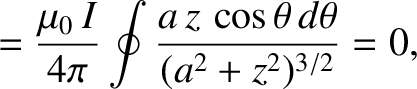
Consider an infinite straight wire, running along the
 -axis, that carries a current . See Figure 2.20.
Let us reconstruct the magnetic field generated by the wire at point
-axis, that carries a current . See Figure 2.20.
Let us reconstruct the magnetic field generated by the wire at point
 using the Biot-Savart
law. Suppose that the perpendicular distance to the wire is
using the Biot-Savart
law. Suppose that the perpendicular distance to the wire is  . It is
easily seen that
. It is
easily seen that
 |
 |
(2.227) |
 |
 |
(2.228) |
 |
 |
(2.229) |
 |
 |
(2.230) |
 is a cylindrical polar coordinate. (See Section A.23.) Hence,
 |
(2.231) |
Thus, according to Equation (2.226), we have
which gives
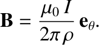 |
(2.233) |
Thus, we conclude that the Biot-Savart law is a more general form of the familiar result (2.206) that is
not restricted to long straight wires.
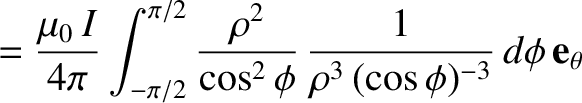
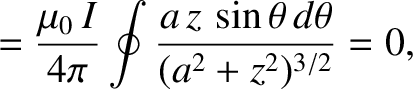
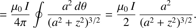
Consider a circular wire loop of radius  that carries a current . Suppose that the loop lies in the
  -
- plane, and is centered on the origin. Let us use the Biot-Savart law to calculate the magnetic field
generated by the coil along a perpendicular axis that passes through its center (i.e., along the -axis).
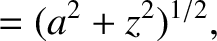
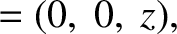
Let be the distance of the
point of observation from the center of the loop, and let the angle parameterize position on the loop. Thus, we have
plane, and is centered on the origin. Let us use the Biot-Savart law to calculate the magnetic field
generated by the coil along a perpendicular axis that passes through its center (i.e., along the -axis).
Let be the distance of the
point of observation from the center of the loop, and let the angle parameterize position on the loop. Thus, we have
where the right-hand sides of the previous two equations are Cartesian components.
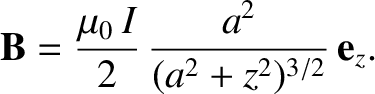
It follows that
 |
 |
(2.236) |
|
 |
(2.237) |
 |
 |
(2.238) |
 |
 |
(2.239) |
 |
(2.243) |
Suppose that we have two identical current loops of radius . Let both loops be centered on
the -axis, and let the first lie in the plane  , and the second in the plane
  . Furthermore,
suppose that a current flows around each loop in the same direction. By the principle of
superposition, making use of the previous equation, the magnetic field generated on the -axis by the two loops is
. Furthermore,
suppose that a current flows around each loop in the same direction. By the principle of
superposition, making use of the previous equation, the magnetic field generated on the -axis by the two loops is
![$\displaystyle B_z = \frac{\mu_0\,I}{2}\left(\frac{a^2}{[a^2+(z-d)^2]^{3/2}} + \frac{a^2}{[a^2+(z+d)^2]^{3/2}}\right).$](img1604.png) |
(2.244) |
If we Taylor expand the previous expression about  then we obtain
![$\displaystyle B_z= \frac{\mu_0\,I}{2}\,\frac{a^2}{(a^2+d^2)^{3/2}}\left\{2 + 3\left[\frac{(2\,d)^2-a^2}{(a^2+d^2)^2}\right]z^2+{\cal O}(z^4)\right\}.$](img1606.png) |
(2.245) |
Suppose that we wish to make the magnetic field in the region between the loops as uniform as possible.
We can clearly achieve this goal if we adjust the spacing  between the loops in such a manner
that the coefficient of
between the loops in such a manner
that the coefficient of  in the previous expression is set to zero. In this case, the leading order non-constant
term in the expansion is
in the previous expression is set to zero. In this case, the leading order non-constant
term in the expansion is
 . It can be seen that
we need
. It can be seen that
we need  . In other words, the spacing between the loops must equal the radius of the loops. The approximately
uniform magnetic field between the loops becomes
. In other words, the spacing between the loops must equal the radius of the loops. The approximately
uniform magnetic field between the loops becomes
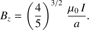 |
(2.246) |
A pair of current loops set up in this manner are known as Helmholtz coils.
Finally, we can generalize the Biot-Savart law, (2.226), to determine the magnetic field generated by a
distributed current of density
 by making the identification
 |
(2.247) |
Thus, we obtain
 |
(2.248) |
where the volume integral is taken over all space.

![$\displaystyle =\frac{\mu_0 \,I}{4\pi \,\rho} \int_{-\pi/2}^{\pi/2} \cos\phi\,d\...
...mu_0 \,I}{4\pi \,\rho} \left[ \sin\phi\right]_{-\pi/2}^{\pi/2}\,{\bf e}_\theta,$](img1583.png)


![\includegraphics[height=2.75in]{Chapter03/fig3_14.eps}](img1571.png)