We saw in Equation (2.16) that
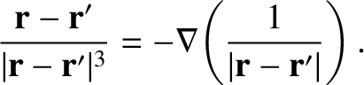 |
(2.249) |
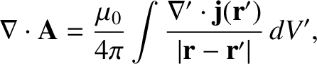
This equation can be combined with the generalized Biot-Savart law, (2.248), to give
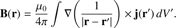 |
(2.250) |
It follows that
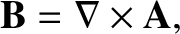 |
(2.251) |
where
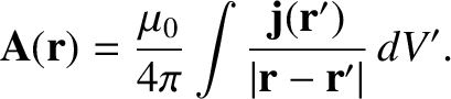 |
(2.252) |
(See Section A.24.)
Here, the vector field
 is known as the magnetic vector potential.
It is possible to prove that the
magnetic vector potential defined in the previous equation is a divergence-free field.
Note that
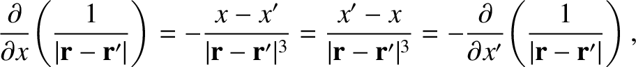 |
(2.253) |
which implies that
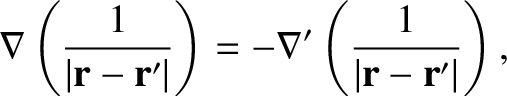 |
(2.254) |
where  is the operator
 . (See Section A.19.) Taking the divergence of Equation (2.252), and making use of
the previous relation, we obtain
. (See Section A.19.) Taking the divergence of Equation (2.252), and making use of
the previous relation, we obtain
 |
(2.255) |
Now,
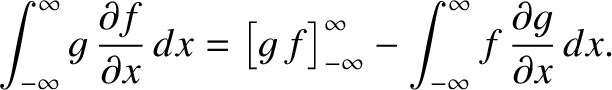 |
(2.256) |
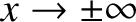
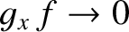
However, if
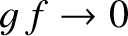 as
as
 then we can neglect the
first term on the right-hand side of the previous equation, and write
then we can neglect the
first term on the right-hand side of the previous equation, and write
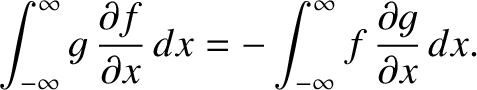 |
(2.257) |
A simple generalization of this result yields
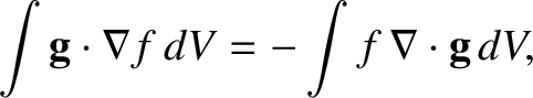 |
(2.258) |
provided that
 as
as
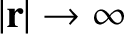 , etc cetera.
Thus, Equation (2.255)
yields
, etc cetera.
Thus, Equation (2.255)
yields
 |
(2.259) |
provided that
 is bounded as
. Now, the flux of electric charge out of a surface
is bounded as
. Now, the flux of electric charge out of a surface  , enclosing a volume
  , is
, is
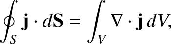 |
(2.260) |
where use has been made of the divergence theorem. (See Section A.20.)
However, for a steady current distribution, this flux must be zero, otherwise positive or negative electric
charge would build up inside . Moreover, the flux must be zero for all possible volumes, , which implies that
 |
(2.261) |
for a steady current distribution. Hence, we deduce from Equation (2.259) that
 |
(2.262) |
for a steady current distribution.