Next: Electric Potential Energy Up: Electrostatic Fields Previous: Electric Field
 and
and
 in Cartesian coordinates.
The
in Cartesian coordinates.
The  -component of
 is
written
is
written
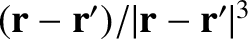
![$\displaystyle \frac{x - x'}{[(x-x')^2+(y-y')^2 + (z-z')^2]^{\,3/2}}.$](img1147.png) |
(2.14) |
![$\displaystyle \frac{x - x'}{[(x-x')^2+(y-y')^2 + (z-z')^2]^{\,3/2}} =$](img1148.png) |
||
![$\displaystyle -\frac{\partial}{\partial x}\!\left(
\frac{1}{[(x-x')^2+(y-y')^2 + (z-z')^2]^{\,1/2}}\right).$](img1149.png) |
(2.15) |
 denotes differentiation with respect to at constant
  ,
,  ,
,  ,
,  , and
, and  .
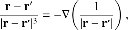
Because there is nothing special about the -axis, we can write
where
.
Because there is nothing special about the -axis, we can write
where
 is a differential operator that involves the components of
  , but not
those of
, but not
those of  . (See Section A.19.)
It follows from Equation (2.13) that
where
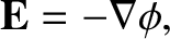
Thus, we conclude that the electric field,
. (See Section A.19.)
It follows from Equation (2.13) that
where
Thus, we conclude that the electric field,
 , generated by a collection of fixed electric charges can be written
as minus the gradient of a scalar field,
, generated by a collection of fixed electric charges can be written
as minus the gradient of a scalar field,
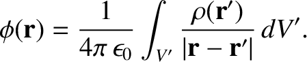
 —known as the electric scalar potential—and that this scalar field can be expressed as a
simple volume integral involving the electric charge distribution.
—known as the electric scalar potential—and that this scalar field can be expressed as a
simple volume integral involving the electric charge distribution.
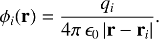
The scalar potential generated by an electric charge  located at the origin is
 |
(2.19) |
 is a spherical polar coordinate. (See Section A.23.)
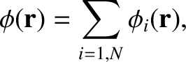
Moreover, according to Equations (2.11) and (2.16), the scalar potential generated by a set of
is a spherical polar coordinate. (See Section A.23.)
Moreover, according to Equations (2.11) and (2.16), the scalar potential generated by a set of  discrete charges
  , located at displacements
  , is
where
Thus, the net scalar potential is just the sum of the potentials generated by each
of the charges taken in isolation.
, is
where
Thus, the net scalar potential is just the sum of the potentials generated by each
of the charges taken in isolation.