Next: Electric Scalar Potential Up: Electrostatic Fields Previous: Coulomb's Law
 point electric charges. Let the
  th charge have electric charge
  and displacement
  .
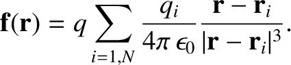
As is the case for gravitational forces (see Section 1.8.1), it is an experimentally demonstrated fact that electrical forces are superposable; that is, the electrical force acting on a test charge whose electric charge is
.
As is the case for gravitational forces (see Section 1.8.1), it is an experimentally demonstrated fact that electrical forces are superposable; that is, the electrical force acting on a test charge whose electric charge is
 and whose displacement is
  is simply the sum of all of the
Coulomb-law forces exerted on it by each of the other charges taken in isolation. In other
words, the electrical force exerted by the th charge (say) on the test charge is
the same as if all of the other charges were not present. Thus, generalizing Equation (2.2), the force acting
on the test charge is given by
is simply the sum of all of the
Coulomb-law forces exerted on it by each of the other charges taken in isolation. In other
words, the electrical force exerted by the th charge (say) on the test charge is
the same as if all of the other charges were not present. Thus, generalizing Equation (2.2), the force acting
on the test charge is given by
 |
(2.9) |
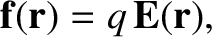
It is helpful to introduce a vector field,
 , known as the
electric field, which is defined as the force exerted on a test charge of unit electric charge whose displacement is . Thus, from the previous equation, the electrical force on a test charge whose displacement is is written
, known as the
electric field, which is defined as the force exerted on a test charge of unit electric charge whose displacement is . Thus, from the previous equation, the electrical force on a test charge whose displacement is is written
According to the previous equation, the electric field generated by a single point electric charge located at the origin is purely radial,
is directed outward if the charge is positive, and inward if it is negative, and has
magnitude
 is a spherical polar coordinate. Moreover,
  is the radial component of the field in spherical polar coordinates.
The other components are zero. (See Section A.23.)
We can represent an electric field by so-called field-lines.
The direction of the lines
indicates
the direction of the
local electric field, and the density of the lines perpendicular to this direction
is proportional to the magnitude of the local electric field.
It follows from Equation (2.12) that the number of field-lines crossing the
surface of a sphere centered on a point charge (which is equal to
times the area,
is the radial component of the field in spherical polar coordinates.
The other components are zero. (See Section A.23.)
We can represent an electric field by so-called field-lines.
The direction of the lines
indicates
the direction of the
local electric field, and the density of the lines perpendicular to this direction
is proportional to the magnitude of the local electric field.
It follows from Equation (2.12) that the number of field-lines crossing the
surface of a sphere centered on a point charge (which is equal to
times the area,  , of the surface) is independent
of the radius of the sphere.
Thus, the field of a point positive electric charge is represented by a group of equally-spaced, unbroken, straight-lines radiating from the charge. See Figure 2.1.
Likewise, field of a point negative charge is represented by a group of
equally-spaced, unbroken, straight-lines converging on the charge.
, of the surface) is independent
of the radius of the sphere.
Thus, the field of a point positive electric charge is represented by a group of equally-spaced, unbroken, straight-lines radiating from the charge. See Figure 2.1.
Likewise, field of a point negative charge is represented by a group of
equally-spaced, unbroken, straight-lines converging on the charge.
Because electrical forces are superposable, it follows that electric fields are also
superposable.
In other words, the electric
field generated by a collection of electric charges is
simply the sum of the fields
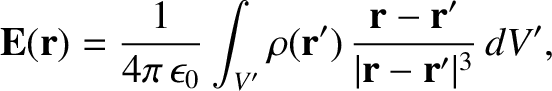
generated by each of the charges taken in isolation. Suppose that, instead of having a collection of discrete electric charges, we
have a continuous distribution of charge represented by an electric charge density
 . Thus, the electric charge at displacement
  is
is
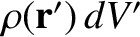 , where
  is the volume element
at . It follows from a straight-forward extension of Equation (2.11) that the electric
field generated by this charge distribution is
is the volume element
at . It follows from a straight-forward extension of Equation (2.11) that the electric
field generated by this charge distribution is
 , that contains all of the charges.
![\includegraphics[height=2.5in]{Chapter03/fig3_2.eps}](img1138.png)