Next: Circuits Up: Magnetic Induction Previous: Inductance
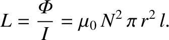
 , and radius
  ,
that has
,
that has  turns per unit length,
and carries a current
turns per unit length,
and carries a current  . The longitudinal (i.e., directed along the
axis of the solenoid) magnetic field within the solenoid is approximately uniform,
and is given by
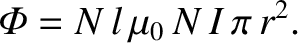
(See Section 2.2.11.) The magnetic flux passing though each turn of the solenoid wire is
. The longitudinal (i.e., directed along the
axis of the solenoid) magnetic field within the solenoid is approximately uniform,
and is given by
(See Section 2.2.11.) The magnetic flux passing though each turn of the solenoid wire is
 . Thus, the total flux passing through
the solenoid wire, which has
. Thus, the total flux passing through
the solenoid wire, which has  turns, is
 |
(2.323) |
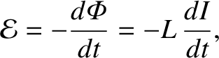
Suppose that the current flowing through the solenoid changes.
A change in the current implies a change in the magnetic flux linking the solenoid
wire, because
 . According to Faraday's
law, this change
generates an emf in the wire. By Lenz's law, the emf is such
as to oppose the change in the current; that is, it is a back-emf. Thus, we can write
. According to Faraday's
law, this change
generates an emf in the wire. By Lenz's law, the emf is such
as to oppose the change in the current; that is, it is a back-emf. Thus, we can write
 is the generated back-emf. [See Equation (2.284).]
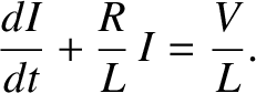
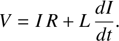
Suppose that our solenoid has an electrical resistance  . Let us
connect the ends of the solenoid across the terminals of a battery of
constant voltage
. Let us
connect the ends of the solenoid across the terminals of a battery of
constant voltage  . The equivalent circuit is shown in Figure 2.27.
The inductance and resistance of the solenoid are represented by a perfect
inductor,
. The equivalent circuit is shown in Figure 2.27.
The inductance and resistance of the solenoid are represented by a perfect
inductor,  , and a perfect resistor, , connected in series. The voltage drop
across the inductor and resistor is equal to the voltage of the battery,
. The voltage drop across the resistor is simply
, and a perfect resistor, , connected in series. The voltage drop
across the inductor and resistor is equal to the voltage of the battery,
. The voltage drop across the resistor is simply  (see Section 2.1.11), whereas the
voltage drop across the inductor (i.e., minus the back-emf) is
(see Section 2.1.11), whereas the
voltage drop across the inductor (i.e., minus the back-emf) is
 . Here, is the current flowing through the solenoid.
It follows that
. Here, is the current flowing through the solenoid.
It follows that
. We can rearrange it to
give
 |
(2.327) |
 |
(2.328) |
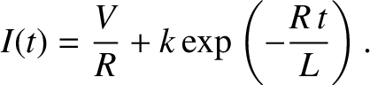
 is fixed by the initial conditions. Suppose that the
battery is connected at time
is fixed by the initial conditions. Suppose that the
battery is connected at time  , when
  . It follows that
  , so
that
This curve is shown in Figure 2.28.
It can be seen that, after the battery is connected, the current
ramps up, and attains its steady-state value
, so
that
This curve is shown in Figure 2.28.
It can be seen that, after the battery is connected, the current
ramps up, and attains its steady-state value  (which comes from Ohm's
law), on the characteristic timescale
(which comes from Ohm's
law), on the characteristic timescale
 |
(2.330) |
 , and to more than 99%
of its final value at time
, and to more than 99%
of its final value at time  .
The timescale
.
The timescale  is sometimes called the time constant of the circuit, or
(somewhat unimaginatively) the L over R time of the circuit. We conclude that it takes a finite time to
establish a steady current flowing through a solenoid.
is sometimes called the time constant of the circuit, or
(somewhat unimaginatively) the L over R time of the circuit. We conclude that it takes a finite time to
establish a steady current flowing through a solenoid.
![\includegraphics[height=3in]{Chapter03/fig7_3.eps}](img1770.png) |
![\includegraphics[height=2.5in]{Chapter03/fig7_2.eps}](img1756.png)
![$\displaystyle I(t) = \frac{V}{R} \left[1-\exp\left(-\frac{R\,t}{L}\right)\right].$](img1765.png)