Next: Electric Scalar Potential Up: Magnetic Induction Previous: Magnetic Induction
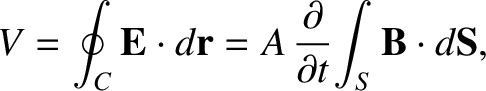
Prior to 1830, the only known way in which to cause an electric current to flow through a conducting wire was to connect the ends of the wire to the positive and negative terminals of a battery. We measure a battery's ability to push current down a wire in terms of its voltage, by which we mean the voltage difference between its positive and negative terminals. Of course, volts are the units used to measure electric scalar potential, so when we talk about a 6 V battery, what we are really saying is that the difference in electric scalar potential between its positive and negative terminals is six volts. This insight allows us to write
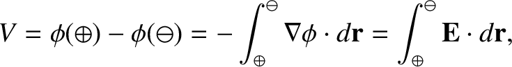 |
(2.280) |
 is the battery voltage,
  denotes the positive terminal,
 the negative terminal, and
  is an element of length along the
wire. Of course, the previous equation is a direct consequence of
is an element of length along the
wire. Of course, the previous equation is a direct consequence of
 . [See Equation (2.17) and Section A.18.] Clearly, a voltage difference between two ends of a wire
attached to a battery implies
the presence of a longitudinal electric field that pushes electric charges along the
wire. This field is directed from the positive terminal of the battery to the negative
terminal, and is, therefore, such as to force electrons to flow through the
wire from the negative to the positive terminal. As expected, this implies that
a net
positive current flows from the positive to the negative terminal. The fact that
. [See Equation (2.17) and Section A.18.] Clearly, a voltage difference between two ends of a wire
attached to a battery implies
the presence of a longitudinal electric field that pushes electric charges along the
wire. This field is directed from the positive terminal of the battery to the negative
terminal, and is, therefore, such as to force electrons to flow through the
wire from the negative to the positive terminal. As expected, this implies that
a net
positive current flows from the positive to the negative terminal. The fact that
 is a conservative field (i.e.,
) ensures that the voltage difference, ,
is independent of the
path of the wire between the terminals. In other words, two different wires attached to the same battery
develop identical voltage differences.
is a conservative field (i.e.,
) ensures that the voltage difference, ,
is independent of the
path of the wire between the terminals. In other words, two different wires attached to the same battery
develop identical voltage differences.
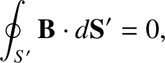
Let us now consider a closed loop of wire (with no battery). The voltage around such a loop, which is sometimes called the electromotive force, or emf, is
 |
(2.281) |
 and the curl theorem. [See Equations (2.17) and (2.25), and Section A.22.]
We conclude that, because is a conservative field (i.e.,
), the emf around a
closed loop of wire
is automatically zero, and so there is no current flow around such a loop.
and the curl theorem. [See Equations (2.17) and (2.25), and Section A.22.]
We conclude that, because is a conservative field (i.e.,
), the emf around a
closed loop of wire
is automatically zero, and so there is no current flow around such a loop.
However, in 1830, Michael Faraday discovered that a changing magnetic field can cause a current to flow around a closed loop of wire (in the absence of a battery). Of course, if current flows around the loop then there must be an emf. In other words,
 |
(2.282) |
is not a conservative field, and that
 . Clearly, we are going to have to modify some
of our ideas regarding electric fields.
. Clearly, we are going to have to modify some
of our ideas regarding electric fields.
Faraday continued his experiments, and found that
another way of generating an emf around a loop of wire
is to keep the magnetic field constant
and to move the loop. (See Section 2.3.9.) Eventually, Faraday was able to
formulate a law that accounted for all of his experiments; the emf
generated around a loop of wire in a magnetic field is proportional to
the rate of change of the flux of the magnetic field through the loop. (See Section A.20.) Thus,
if the loop is denoted  , and
, and  is some surface attached to the loop, then Faraday's
experiments can be summed up by writing
is some surface attached to the loop, then Faraday's
experiments can be summed up by writing
 is a constant of proportionality.
Thus, the changing flux of the magnetic field
passing through the loop
generates an electric field directed around the loop. This process is know as
magnetic induction.
is a constant of proportionality.
Thus, the changing flux of the magnetic field
passing through the loop
generates an electric field directed around the loop. This process is know as
magnetic induction.
SI units have been carefully chosen so as to make  in
the previous equation. So, the only question that we now have to answer is whether
in
the previous equation. So, the only question that we now have to answer is whether
 or
or  . In other words, we need to decide which way around the loop the induced emf
drives the current. We possess a general principle, known as
Le Chatelier's principle, that allows us to
answer such questions. According to Le Chatelier's principle, every change
in a physical system generates a reaction that acts to minimize the change. Essentially, this implies
that the universe is stable to small perturbations. When Le Chatelier's principle
is applied to the particular case of
magnetic induction, it is usually called Lenz's law, after Emil Lenz who formulated it in 1834. According to Lenz's
law, the current induced by an emf around a closed loop
is always such that the magnetic field it produces acts to counteract the
change in magnetic flux that generates the emf.
From Figure 2.25, it is clear that if the magnetic field
. In other words, we need to decide which way around the loop the induced emf
drives the current. We possess a general principle, known as
Le Chatelier's principle, that allows us to
answer such questions. According to Le Chatelier's principle, every change
in a physical system generates a reaction that acts to minimize the change. Essentially, this implies
that the universe is stable to small perturbations. When Le Chatelier's principle
is applied to the particular case of
magnetic induction, it is usually called Lenz's law, after Emil Lenz who formulated it in 1834. According to Lenz's
law, the current induced by an emf around a closed loop
is always such that the magnetic field it produces acts to counteract the
change in magnetic flux that generates the emf.
From Figure 2.25, it is clear that if the magnetic field  is
increasing and the current
is
increasing and the current  circulates clockwise (as seen from above) then
the current generates a field
circulates clockwise (as seen from above) then
the current generates a field  that opposes the increase in the magnetic flux
through the loop, in
accordance with Lenz's law. The direction of the current is opposite to the
sense of circulation of the current loop , as determined by the right-hand rule (assuming that the flux of through the
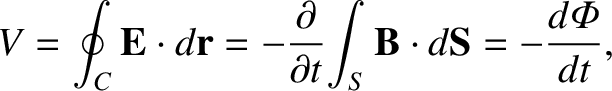
loop is positive), so this implies that in Equation (2.283). Thus, Faraday's
law takes the form
that opposes the increase in the magnetic flux
through the loop, in
accordance with Lenz's law. The direction of the current is opposite to the
sense of circulation of the current loop , as determined by the right-hand rule (assuming that the flux of through the
loop is positive), so this implies that in Equation (2.283). Thus, Faraday's
law takes the form
 is the magnetic flux through the loop.
Experimentally, Faraday's law is found to correctly predict the emf
(i.e.,
 ) generated around any wire loop, irrespective of
the position or shape of the loop.
It is reasonable to assume that the same emf would be
generated in the absence of the wire (of course, no current would flow
in this case). We conclude that Equation (2.284) is valid for any closed loop . Now, if Faraday's
law is to make sense then it must hold for all surfaces, , attached to the
loop, . Clearly, if the flux of the magnetic field through the loop depends on
the surface upon which it is evaluated then Faraday's law is going to predict
different emfs for different surfaces. Because there is no preferred surface for
a general non-coplanar loop, this would not make any sense. The condition
for the flux of the magnetic field,
) generated around any wire loop, irrespective of
the position or shape of the loop.
It is reasonable to assume that the same emf would be
generated in the absence of the wire (of course, no current would flow
in this case). We conclude that Equation (2.284) is valid for any closed loop . Now, if Faraday's
law is to make sense then it must hold for all surfaces, , attached to the
loop, . Clearly, if the flux of the magnetic field through the loop depends on
the surface upon which it is evaluated then Faraday's law is going to predict
different emfs for different surfaces. Because there is no preferred surface for
a general non-coplanar loop, this would not make any sense. The condition
for the flux of the magnetic field,
 , to depend
only on the loop to which the surface is attached, and not on the nature
of the surface itself, is
, to depend
only on the loop to which the surface is attached, and not on the nature
of the surface itself, is
 . (See Section A.20.)
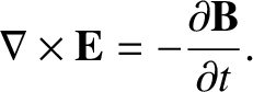
Faraday's law, Equation (2.284), can be converted into a field equation using the curl theorem. (See Section A.22.) We obtain
This field equation describes how a changing magnetic field generates an electric field. The divergence theorem (see Section A.20) applied to Equation (2.285) gives the familiar field equation |
(2.287) |
The divergence of Equation (2.286) yields
 |
(2.288) |
 . (See Section A.22.)
Thus, the field equation (2.286) actually demands that the divergence of the
magnetic field must be constant in time for self-consistency (this implies
that the flux of the magnetic field through a loop need not be a well defined
quantity, as long as
its time derivative is well defined). However, a constant
non-solenoidal magnetic field can only be generated by magnetic monopoles,
and magnetic monopoles do not exist (as far as we are aware). (See Section 2.2.9.) Hence,
. (See Section A.22.)
Thus, the field equation (2.286) actually demands that the divergence of the
magnetic field must be constant in time for self-consistency (this implies
that the flux of the magnetic field through a loop need not be a well defined
quantity, as long as
its time derivative is well defined). However, a constant
non-solenoidal magnetic field can only be generated by magnetic monopoles,
and magnetic monopoles do not exist (as far as we are aware). (See Section 2.2.9.) Hence,
 .
.
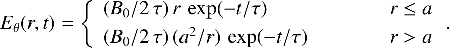
As an example of the use of Faraday's law, let us calculate the electric
field generated by a decaying magnetic field of the form
 , where
![\begin{displaymath}B_z(r,t) = \left\{
\begin{array}{lcc}
B_0\,\exp(-t/\tau)&\mbox{\hspace{1cm}}&r\leq a\\ [0.5ex]
0&&r>a
\end{array}\right.,\end{displaymath}](img1694.png) |
(2.289) |
 is a cylindrical polar coordinate. (See Section A.23.)
Here,
is a cylindrical polar coordinate. (See Section A.23.)
Here,  and
and  are positive constants.
By symmetry, we expect an induced electric field of the form
are positive constants.
By symmetry, we expect an induced electric field of the form
 .
We also expect
.
We also expect
 , because there are no electric charges
in the problem. [See Equation (2.54).] This rules out a radial electric field. We can also rule
out a
, because there are no electric charges
in the problem. [See Equation (2.54).] This rules out a radial electric field. We can also rule
out a  -directed electric field, because
![$\nabla\times [E_z(r)\,{\bf e}_z] = -(\partial E_z/\partial r)\,{\bf e}_\theta$](img1697.png) , and we require
, and we require
 . Hence, the induced electric field must be of the
form
. Hence, the induced electric field must be of the
form
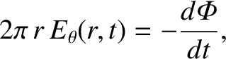
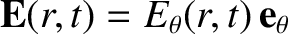 . Now, according to
Faraday's law, (2.284), the line integral of the electric field around some closed
loop is equal to minus the rate of change of the magnetic flux passing through
the loop. If we choose a loop that is a circle of radius in the
. Now, according to
Faraday's law, (2.284), the line integral of the electric field around some closed
loop is equal to minus the rate of change of the magnetic flux passing through
the loop. If we choose a loop that is a circle of radius in the  -
- plane then we have
 |
(2.290) |
 is the flux of the magnetic field (in the
  direction) passing through a circular loop of radius .
It is evident that
direction) passing through a circular loop of radius .
It is evident that
![\begin{displaymath}{\mit\Phi}(r,t) = \left\{
\begin{array}{lcc}
\pi\,r^2\,B_0\,\...
...\ [0.5ex]
\pi\,a^2\,B_0\,\exp(-t/\tau)&&r>a
\end{array}\right..\end{displaymath}](img1701.png) |
(2.291) |
 |
(2.292) |
![\includegraphics[height=2.5in]{Chapter03/fig4_1.eps}](img1686.png)