Gauss's Law
Consider a single electric charge  located at the origin. The electric field generated by
such a charge is given by Equation (2.12). Suppose that we surround the charge by
a concentric spherical surface
located at the origin. The electric field generated by
such a charge is given by Equation (2.12). Suppose that we surround the charge by
a concentric spherical surface  of radius
  . See Figure 2.2. The flux of the
electric field through this surface is
given by
. See Figure 2.2. The flux of the
electric field through this surface is
given by
 |
(2.28) |
because the normal to the surface is always
parallel to the local electric field. (See Section A.16.) Here, is also a spherical polar coordinate. (See Section A.23.)
However, we also know from the divergence theorem that
 |
(2.29) |
where  is the volume enclosed by surface . (See Section A.20.) Let us evaluate
 directly. In Cartesian coordinates, the electric field (2.12) is written
 |
(2.30) |
where
 . So,
. So,
 |
(2.31) |
Here, use has been made of the easily demonstrated result
 |
(2.32) |
Formulae analogous to Equation (2.31) can be obtained for
 and
and
 .
The divergence of the field is, thus, given by
.
The divergence of the field is, thus, given by
 |
(2.33) |
(See Section A.20.)
This is an extremely puzzling result. We have from Equations (2.28) and (2.29) that
 |
(2.34) |
and yet we have just proved that
 . This paradox can be
resolved after a close examination of Equation (2.33). At the origin
(
. This paradox can be
resolved after a close examination of Equation (2.33). At the origin
( ), we find that
 , which implies that
can take any value at this point.
Thus, Equations (2.33) and (2.34) can be reconciled
if
is some sort
of “spike” function; that is, if it is zero everywhere, except arbitrarily
close to the origin,
where it becomes very large. This
must occur in such a manner that the volume integral over the spike
is finite.
, which implies that
can take any value at this point.
Thus, Equations (2.33) and (2.34) can be reconciled
if
is some sort
of “spike” function; that is, if it is zero everywhere, except arbitrarily
close to the origin,
where it becomes very large. This
must occur in such a manner that the volume integral over the spike
is finite.
Let us examine how we might construct a one-dimensional spike function.
Consider the “box-car” function
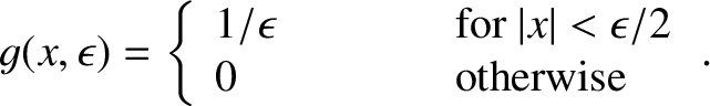 |
(2.35) |
See Figure 2.3.
It is clear that
 |
(2.36) |
Now, consider the function
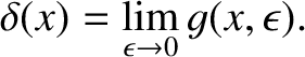 |
(2.37) |
This function is zero everywhere, except arbitrarily close to  , where it is very large.
However, according to Equation (2.36),
the function still possess a finite integral:
, where it is very large.
However, according to Equation (2.36),
the function still possess a finite integral:
 |
(2.38) |
Thus,  has all of the required properties of a spike function.
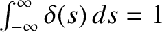
The one-dimensional spike function is called the
Dirac delta function, after Paul Dirac who
invented it in 1927 while investigating quantum mechanics. The delta function is an
example of what mathematicians call a generalized function; it is not
well defined at , but its integral is nevertheless well defined.
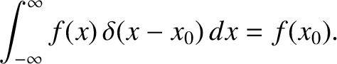
Consider the integral
has all of the required properties of a spike function.
The one-dimensional spike function is called the
Dirac delta function, after Paul Dirac who
invented it in 1927 while investigating quantum mechanics. The delta function is an
example of what mathematicians call a generalized function; it is not
well defined at , but its integral is nevertheless well defined.
Consider the integral
 |
(2.39) |
where  is a function that is well behaved in the vicinity of .
Because the delta function is zero everywhere, apart from arbitrarily close
to , it is clear that
is a function that is well behaved in the vicinity of .
Because the delta function is zero everywhere, apart from arbitrarily close
to , it is clear that
 |
(2.40) |
where use has been made of Equation (2.38). A simple change of variables allows us to define
 , which is
a delta function centered on
, which is
a delta function centered on  . Equation (2.40) gives
 |
(2.41) |
Figure 2.3:
A box-car function.
|
|
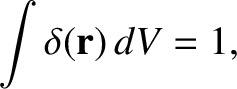
We actually require a three-dimensional delta function; that is, a function
that is zero everywhere,
apart from arbitrarily close to the origin, where it is very large, and whose volume integral is unity.
If we denote this function by
 then it is easily seen that
the three-dimensional delta function is the product of three one-dimensional
delta functions:
then it is easily seen that
the three-dimensional delta function is the product of three one-dimensional
delta functions:
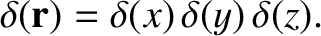 |
(2.42) |
This function is clearly zero everywhere, except arbitrarily close the origin, where it is very large. But, is its volume
integral unity? Let us integrate over a cube of dimension  that is
centered on the origin, and aligned along the Cartesian axes. This
volume integral is obviously separable, so that
that is
centered on the origin, and aligned along the Cartesian axes. This
volume integral is obviously separable, so that
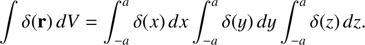 |
(2.43) |
(See Section A.17.)
The integral can be turned into an integral over all space by taking
the limit
 . However, we know that, for one-dimensional
delta functions,
. However, we know that, for one-dimensional
delta functions,
 , so it follows
from the previous equation that
, so it follows
from the previous equation that
 |
(2.44) |
which is the desired result. A simple generalization of previous arguments yields
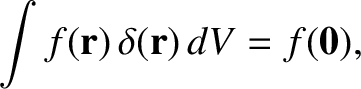 |
(2.45) |
where
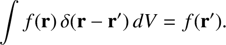
 is any well-behaved scalar field. Finally, we can change variables
and write
is any well-behaved scalar field. Finally, we can change variables
and write
 |
(2.46) |
which is a three-dimensional delta function centered on
 . It is easily demonstrated that
 |
(2.47) |
Up to now, we have only considered volume integrals taken
over all space. However, it
should be obvious that the previous result also holds for integrals
over any finite volume that contains the point
. Likewise,
the integral is zero if does not contain the point
.
Let us now return to the problem in hand. The electric field generated by an electric charge
located at the origin has
everywhere apart from the
origin, and also satisfies
 |
(2.48) |
for a spherical volume centered on the origin. These two facts imply that
 |
(2.49) |
where use has been made of Equation (2.44).
Consider, again, an electric charge located at the origin, and surrounded by a spherical surface
that is centered on the origin. We have seen that the flux of the electric field out of is
 .
Suppose that we now displace the surface , so that it is no longer centered
on the origin. What now is the flux of the electric field out of S? We have
.
Suppose that we now displace the surface , so that it is no longer centered
on the origin. What now is the flux of the electric field out of S? We have
 |
(2.50) |
from the divergence theorem (see Section A.20),
as well as Equation (2.49).
From these two equations,
it is clear that the flux of  out of is still
, as long as the
displacement is not large enough that the origin is no longer enclosed by
the sphere.
Suppose that the surface is not spherical, but is
instead highly distorted. What now is the flux of out of ? As before, the divergence theorem and Equation (2.49) tell us that
the flux remains
, provided that the surface contains the origin. Moreover, this result is completely independent of the shape of .
out of is still
, as long as the
displacement is not large enough that the origin is no longer enclosed by
the sphere.
Suppose that the surface is not spherical, but is
instead highly distorted. What now is the flux of out of ? As before, the divergence theorem and Equation (2.49) tell us that
the flux remains
, provided that the surface contains the origin. Moreover, this result is completely independent of the shape of .
Let us try to extend the previous result. Consider  electric charges
  located at displacements
  . A simple generalization of
Equation (2.49) gives
. A simple generalization of
Equation (2.49) gives
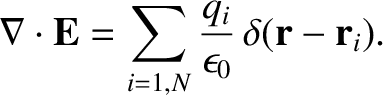 |
(2.51) |
Thus, Equation (2.50) and the previous equation imply that
 |
(2.52) |
where  is the total charge enclosed by the surface . This result is called
Gauss's law, and does
not depend on the shape of the surface. Note that the previous equation is analogous in form to the gravitational
version of Gauss's law, (1.245). This is not surprising because, as we previously mentioned, Gauss's law holds for any inverse-square force law.
is the total charge enclosed by the surface . This result is called
Gauss's law, and does
not depend on the shape of the surface. Note that the previous equation is analogous in form to the gravitational
version of Gauss's law, (1.245). This is not surprising because, as we previously mentioned, Gauss's law holds for any inverse-square force law.
Suppose, finally, that instead of having a set of discrete electric charges, we have a
continuous charge distribution described by a charge density
 .
The charge contained in a small rectangular volume of dimensions
.
The charge contained in a small rectangular volume of dimensions  ,
,  , and
, and  ,
located at displacement
,
located at displacement
 , is
, is
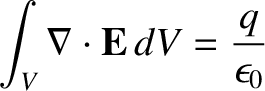
 . However, if we integrate
over this volume element then we obtain
. However, if we integrate
over this volume element then we obtain
 |
(2.53) |
where use has been made of Equation (2.52). Here, the volume element is assumed to be
sufficiently small that
does not vary significantly across
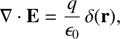
it. Thus, we get
 |
(2.54) |
Equation (2.54) is a differential equation that describes the electric field generated
by a set of charges. We already know the solution to this equation when the
charges are stationary;
it is given by Equation (2.13),
 |
(2.55) |
Incidentally, Equations (2.54) and (2.55) can be reconciled provided
 |
(2.56) |
where use has been made of Equation (2.16). (See Section A.21.)
It follows that
which is the desired result. Here, use has been made of Equation (2.47).
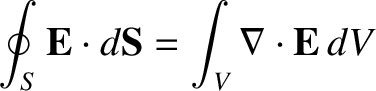
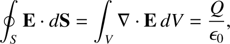
Finally, the most general form of Gauss's law, Equation (2.52),
is obtained by integrating Equation (2.54) over a volume surrounded by
a surface , and making use of
the divergence theorem:
 |
(2.58) |
(See Section A.20.)
![\includegraphics[height=2.5in]{Chapter03/fig3_3.eps}](img1171.png)
![\includegraphics[height=2.5in]{Chapter03/fig3_4.eps}](img1192.png)