Gauss's Law

Gauss's law applies to any inverse-square central force. This law was first discovered by Joseph-Louis Lagrange in 1773, and was later rediscovered by Carl Friedrich Gauss in 1835.

Suppose that we have an isolated point source that emits an incompressible fluid isotropically in all directions at the rate $Q\,({\rm m^3\,s^{-1}})$. By symmetry, we would expect the fluid to flow radially away from the source, isotropically in all directions. In other words, if the source is located at the origin then we expect the fluid velocity at displacement ${\bf r}$ to be of the form

$${\bf v} = v(r)\,\frac{{\bf r}}{r}.$$ (1.242)

Let us surround our source by an imaginary spherical surface of radius $r$. See Figure 1.11. The net volume rate of flow of fluid out of the surface is $4\pi\,r^2\,v(r)$. However, if the fluid is incompressible (and the flow pattern has achieved a steady-state) then the volume rate of flow out of the surface must equal the volume rate of flow from the source (otherwise, the fluid inside the surface would suffer compression or rarefaction). In other words, $4\pi\,r^2\,v(r)=Q$. Hence, Equation (1.242) becomes

$${\bf v} = \frac{Q}{4\pi}\,\frac{{\bf r}}{r^3}.$$ (1.243)

It can be seen that the previous expression has an analogous form to expression (1.241), provided that we make the identifications ${\bf v}\rightarrow {\bf g}$ and $Q\rightarrow -4\pi\,G\,m$.

Figure 1.11: Fluid outflow from a point source.

Suppose that we have $N$ point sources of incompressible fluid. Let the $i$th source have a volume rate of flow $Q_i$. Let us surround these sources by an imaginary closed surface (that is not necessarily spherical), $S$. Now, the volume rate of flow of fluid out of $S$ is $\oint_S {\bf v}\cdot d{\bf S}$, where ${\bf v}({\bf r})$ is the flow field, and $d{\bf S}$ is an (outward pointing) element of $S$. (See Section A.16.) However, if the fluid is incompressible (and the flow pattern has achieved a steady-state) then the volume rate of flow out of $S$ must match the sum of the volume rates of flow of the sources within $S$ (otherwise, the fluid inside the surface would suffer compression or rarefaction). Thus, we deduce that

$$\oint_S {\bf v}\cdot d{\bf S} = \sum_{i=1,N} Q_i.$$ (1.244)

Now, if there are sources that lie outside $S$ then they do not affect the previous relation (because a source outside $S$ gives rise to zero net flow of incompressible fluid out of $S$). Hence, we can interpret the sum in the previous equation as a sum that includes all sources that lie inside $S$, but excludes any sources that lie outside $S$.

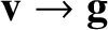
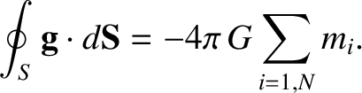
Finally, we can exploit the previously mentioned analogy between incompressible fluid flow and gravitational acceleration to deduce the following result. Suppose that there are $N$ point objects of mass $m_i$. Let us surround these objects by an imaginary surface $S$. Making use of the identifications ${\bf v}\rightarrow {\bf g}$ and $Q_i\rightarrow -4\pi\,G\,m_i$, the previous equation transforms to give

$$\oint_S {\bf g}\cdot d{\bf S} = -4\pi\,G\sum_{i=1,N}m_i.$$ (1.245)

As before, if there are objects outside $S$ then they do not affect the previous relation. Thus, we deduce that the flux of gravitational acceleration out of an arbitrary closed surface, $S$, is equal to $-4\pi\,G$ multiplied by the sum of the masses of any objects lying inside the surface. This is Gauss's law. The imaginary surface $S$ is known as a Gaussian surface.

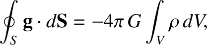
Suppose that, instead of having a collection of point objects, we have a continuous mass distribution whose mass density is $\rho({\bf r})$. The previous equation generalizes to give

$$\oint_S {\bf g}\cdot d{\bf S} = -4\pi\,G\int_V \rho\,dV,$$ (1.246)

where $V$ is the volume enclosed by $S$, and $dV$ is an element of $V$. (See Section A.17.) Now, according to the divergence theorem (see Section A.20),

$$\oint_S {\bf g}\cdot d{\bf S} = \int_V \nabla\cdot {\bf g}\,dV,$$ (1.247)

where $\nabla\cdot {\bf g} = \partial g_x/\partial x+\partial g_y/\partial y + \partial g_z/\partial z$ is the divergence of the acceleration field. The previous two equations yield

$$\int_V \nabla\cdot {\bf g}\,dV= -4\pi\,G\int_V \rho\,dV.$$ (1.248)

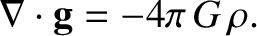
However, the volume $V$ is arbitrary, so the only way that the previous equation could hold for all possible volumes is if

$$\nabla\cdot{\bf g} = - 4\pi\,G\,\rho.$$ (1.249)

This is the differential form of Gauss's law.