Next: Electrostatic Energy Up: Electrostatic Fields Previous: Gauss's Law
 th particle in the
electric field,
th particle in the
electric field,
 , generated by all of the other static particles.
The equilibrium position of the th particle corresponds to some
point of displacement
, generated by all of the other static particles.
The equilibrium position of the th particle corresponds to some
point of displacement  at which
 , because this implies that the particle is not
subject to an electrical force. By implication,
does not correspond to the equilibrium displacement of
any other particle in the system.
However, in order
for to be the displacement of a stable equilibrium point, the th particle
must experience a restoring force when its displacement deviates slightly from in any direction. Assuming that the
th particle is (say) positively charged, this implies that the electric
field must be directed radially toward the point whose displacement is
at all neighboring points. Hence,
if we consider a small sphere centered on displacement then there must be a negative flux of
, because this implies that the particle is not
subject to an electrical force. By implication,
does not correspond to the equilibrium displacement of
any other particle in the system.
However, in order
for to be the displacement of a stable equilibrium point, the th particle
must experience a restoring force when its displacement deviates slightly from in any direction. Assuming that the
th particle is (say) positively charged, this implies that the electric
field must be directed radially toward the point whose displacement is
at all neighboring points. Hence,
if we consider a small sphere centered on displacement then there must be a negative flux of
 through the surface of this sphere. According to Gauss's law, this necessitates the presence of a negative
charge at displacement . However, there is no such charge at displacement .
Hence, we conclude that cannot be directed radially toward the point whose displacement is
at all neighboring points. In other
words, there must be some neighboring points at which is directed away
from the point whose displacement is . Hence, a positively charged particle
placed at displacement can always escape by moving to such neighboring points.
One corollary of Earnshaw's theorem is that classical electrostatics cannot
account for the stability of atoms and molecules.
through the surface of this sphere. According to Gauss's law, this necessitates the presence of a negative
charge at displacement . However, there is no such charge at displacement .
Hence, we conclude that cannot be directed radially toward the point whose displacement is
at all neighboring points. In other
words, there must be some neighboring points at which is directed away
from the point whose displacement is . Hence, a positively charged particle
placed at displacement can always escape by moving to such neighboring points.
One corollary of Earnshaw's theorem is that classical electrostatics cannot
account for the stability of atoms and molecules.
As an example of the use of Gauss's law, let us calculate the electric field
generated by a spherically symmetric charge annulus of inner radius  ,
and outer radius
,
and outer radius  , centered on the origin, and carrying a uniformly
distributed electric charge
, centered on the origin, and carrying a uniformly
distributed electric charge  . Now, by symmetry, we expect a spherically
symmetric charge distribution to generate a spherically symmetric
potential,
. Now, by symmetry, we expect a spherically
symmetric charge distribution to generate a spherically symmetric
potential,  , where
  is a spherical polar coordinate. (See Section A.23.) It therefore follows from Equation (2.17) that the electric field is both
spherically symmetric and radial; that is,
is a spherical polar coordinate. (See Section A.23.) It therefore follows from Equation (2.17) that the electric field is both
spherically symmetric and radial; that is,
 .
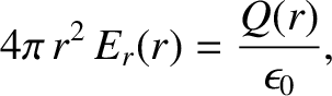
Let us apply Gauss's law to an imaginary spherical surface, of radius
, centered on the origin. See Figure 2.4. Such a surface is generally known as a Gaussian surface. According to
Gauss's law, (2.58), the flux of the electric field out of the surface is equal to
the enclosed charge, divided by
.
Let us apply Gauss's law to an imaginary spherical surface, of radius
, centered on the origin. See Figure 2.4. Such a surface is generally known as a Gaussian surface. According to
Gauss's law, (2.58), the flux of the electric field out of the surface is equal to
the enclosed charge, divided by
 . The flux is easy to calculate because the electric field is everywhere perpendicular to the
surface. We obtain
. The flux is easy to calculate because the electric field is everywhere perpendicular to the
surface. We obtain
 |
(2.59) |
 is the charge enclosed by a Gaussian surface of radius .
However, simple arguments involving proportion reveal that
is the charge enclosed by a Gaussian surface of radius .
However, simple arguments involving proportion reveal that
![\begin{displaymath}Q(r) = \left\{
\begin{array}{lcl}
0&\mbox{\hspace{1cm}}&r<a\\...
...3)\right] Q&&a\leq r\leq b\\ [0.5ex]
Q&&b<r
\end{array}\right..\end{displaymath}](img1229.png) |
(2.60) |
We can easily determine the electric potential associated with the electric field (2.61) using
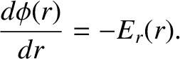 |
(2.62) |
 , and that is
continuous at
, and that is
continuous at  and
and  . (Of course, a discontinuous potential would lead to
an infinite electric field, which is unphysical.) It follows that
. (Of course, a discontinuous potential would lead to
an infinite electric field, which is unphysical.) It follows that
![\begin{displaymath}\phi(r) = \left\{
\begin{array}{lcl}
\left[Q/(4\pi\,\epsilon_...
...eq b\\ [0.5ex]
Q/(4\pi\,\epsilon_0\,r)&&b<r
\end{array}\right..\end{displaymath}](img1236.png) |
(2.63) |
![$\displaystyle W = q\left[\phi(0)-\phi(\infty)\right] = \frac{q\,Q}{4\pi\,\epsilon_0}\,\frac{3}{2}\left(\frac{b^2-a^2}{b^3-a^3}\right).$](img1237.png) |
(2.64) |
![\begin{displaymath}E_r(r) = \left\{
\begin{array}{lcl}
0&\mbox{\hspace{1cm}}&r<a...
... b\\ [0.5ex]
Q/(4\pi\,\epsilon_0\,r^2)&&b<r
\end{array}\right..\end{displaymath}](img1230.png)
![\includegraphics[height=2.5in]{Chapter03/fig3_5.eps}](img1231.png)