Electrostatic Energy
Consider a collection of  static point electric charges
  located at displacements
 .
What is the electrostatic energy stored in such a collection? In other words, how much work would we have to perform in order to assemble
the charges, starting from an initial state in which they are all
at rest and very widely
separated?
.
What is the electrostatic energy stored in such a collection? In other words, how much work would we have to perform in order to assemble
the charges, starting from an initial state in which they are all
at rest and very widely
separated?
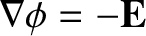
We know that a static electric field is conservative, and can consequently
be written in terms of
a scalar potential:
 |
(2.65) |
[See Equation (2.17).]
We also know that the electrical force acting on a charge  located at displacement
  is
written
is
written
 |
(2.66) |
[See Equation (2.10).]
The work that we would have to do against electrical forces in order to slowly
move the charge from point  to point
  is simply
![$\displaystyle W = \int_P^Q (-{\bf f}) \cdot d{\bf r} =- q \int_P^Q {\bf E} \cdo...
...bf r}
=q\int_P^Q \nabla\phi \cdot d{\bf r} = q \left[ \phi(Q) - \phi(P)\right],$](img1240.png) |
(2.67) |
where  is an element of the path taken between the two points. (See Section 1.3.2.)
The negative sign in the previous expression comes about because we would have to
exert a force
is an element of the path taken between the two points. (See Section 1.3.2.)
The negative sign in the previous expression comes about because we would have to
exert a force  on the charge, in order to counteract the force
exerted by the electric field. Recall, finally, that the scalar potential field
generated by a point charge located at position
on the charge, in order to counteract the force
exerted by the electric field. Recall, finally, that the scalar potential field
generated by a point charge located at position  is
is
 |
(2.68) |
[See Equation (2.21).]
Let us build up our collection of charges one by one. It takes no work to bring the
first charge from infinity, because there is no electric field to fight against.
Let us clamp this charge in position at displacement  . In order to bring the
second charge into position at displacement
. In order to bring the
second charge into position at displacement  ,
we have to do work against the electric field
generated by the first charge. According to Equations (2.67) and (2.68),
this work is given by
,
we have to do work against the electric field
generated by the first charge. According to Equations (2.67) and (2.68),
this work is given by
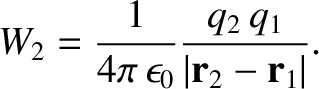 |
(2.69) |
Let us now bring the third charge into position. Because electric fields
and scalar potentials are
superposable, the work done while moving the third charge from infinity to displacement  is simply the sum of the works done against the electric fields generated by
charges 1 and 2, taken in isolation:
is simply the sum of the works done against the electric fields generated by
charges 1 and 2, taken in isolation:
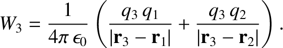 |
(2.70) |
Thus, the total work done in assembling the collection of three charges is given by
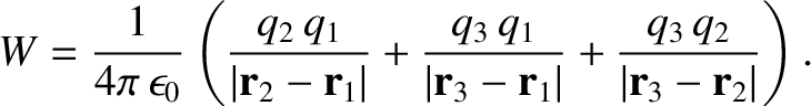 |
(2.71) |
This result can easily be generalized to a collection of charges:
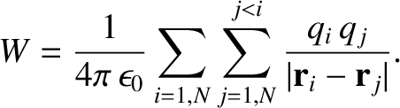 |
(2.72) |
The restriction that  must be less than
  makes the previous summation
rather messy. If we were to sum without restriction (other than
makes the previous summation
rather messy. If we were to sum without restriction (other than  ) then
each pair of charges would be counted twice. It is convenient to do just
this, and then to divide the result by two. Thus, we obtain
) then
each pair of charges would be counted twice. It is convenient to do just
this, and then to divide the result by two. Thus, we obtain
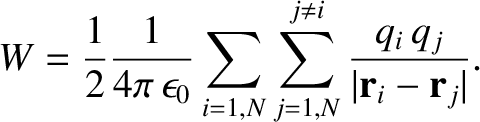 |
(2.73) |
This is the electric potential energy (i.e., the difference between the total energy
and the kinetic energy) of a collection of point electric charges. We can think of this quantity as the
work required to bring stationary charges from infinity and assemble them in the
required formation. Alternatively, it is the kinetic energy that would
be released if the collection were dissolved, and the charges returned to infinity.
But where is this potential energy stored? Let us investigate further.
Equation (2.73) can be written
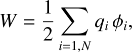 |
(2.74) |
where
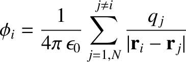 |
(2.75) |
is the scalar potential experienced by the th charge due to the other
charges in the distribution. [See Equation (2.20).]
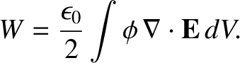
Let us now consider the potential energy of a continuous charge distribution.
It is tempting to write
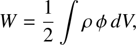 |
(2.76) |
by analogy with Equations (2.74) and (2.75), where
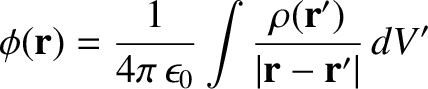 |
(2.77) |
is the familiar scalar potential generated by a continuous charge distribution
of charge density
 [see Equation (2.18)], and where the volume integrals are over all space.
Let us try this scheme out. We know from Equation (2.54) that
[see Equation (2.18)], and where the volume integrals are over all space.
Let us try this scheme out. We know from Equation (2.54) that
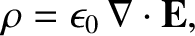 |
(2.78) |
so Equation (2.76) can be written
 |
(2.79) |
Now,
 |
(2.80) |
(See Section A.24.)
However,
 , so we obtain
![$\displaystyle W = \frac{\epsilon_0}{2} \left[\int \nabla\cdot ({\bf E}\,\phi)\,dV
+
\int E^2\,dV\right]$](img1258.png) |
(2.81) |
Application of the divergence theorem (see Section A.20) gives
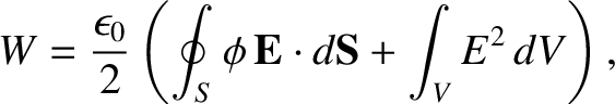 |
(2.82) |
where  is some volume that encloses all of the charges, and
  is its bounding
surface. Let us assume that is a sphere, centered on the origin, and let
us take the limit in which the radius
is its bounding
surface. Let us assume that is a sphere, centered on the origin, and let
us take the limit in which the radius  of this sphere goes to infinity.
We know that, in general, the electric field at large distances from a
bounded charge
distribution looks like the field of a point charge, and, therefore,
falls off like
of this sphere goes to infinity.
We know that, in general, the electric field at large distances from a
bounded charge
distribution looks like the field of a point charge, and, therefore,
falls off like  . Likewise, the potential falls off like
  . (See Section 2.1.7.) However,
the surface area of the sphere increases like
. (See Section 2.1.7.) However,
the surface area of the sphere increases like  . Hence, it is clear that, in the
limit as
. Hence, it is clear that, in the
limit as
 , the surface integral in Equation (2.82) falls off
like , and is consequently zero.
Thus, Equation (2.82) reduces to
, the surface integral in Equation (2.82) falls off
like , and is consequently zero.
Thus, Equation (2.82) reduces to
 |
(2.83) |
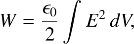
where the volume integral is over all space. This is a very interesting
result. It tells us that the potential energy of a continuous charge
distribution is stored in the electric field generated by that distribution. Of course, we now have to assume that
an electric field possesses an energy density
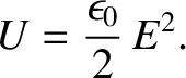 |
(2.84) |
Incidentally, the fact that an electric field possess an energy density demonstrates that it has a real physical existence, and
is not just an aid to the calculation of electrostatic forces.
We can easily check that Equation (2.83) is correct. Suppose that we have an electric
charge that is uniformly distributed within a sphere of
radius  centered on the origin. Let us imagine building up this charge distribution
from a succession of thin spherical layers of infinitesimal thickness. At each
stage, we gather a small amount of charge
centered on the origin. Let us imagine building up this charge distribution
from a succession of thin spherical layers of infinitesimal thickness. At each
stage, we gather a small amount of charge  from infinity, and spread it
over the surface of the sphere in a thin
layer extending from to
from infinity, and spread it
over the surface of the sphere in a thin
layer extending from to  . We continue this process until the final radius of the
sphere is . If
. We continue this process until the final radius of the
sphere is . If  is the sphere's charge when it has attained radius
then the work done in bringing a charge to its surface is
is the sphere's charge when it has attained radius
then the work done in bringing a charge to its surface is
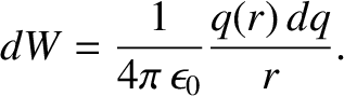 |
(2.85) |
This follows from Equation (2.69), because the electric field generated outside a spherical charge
distribution
is the same as that of a point charge located at its geometric center
( ). (See Section 2.1.7.) If the constant charge density of the sphere is
 then
then
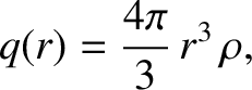 |
(2.86) |
and
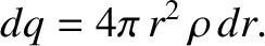 |
(2.87) |
Thus, Equation (2.85) becomes
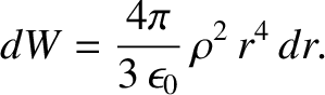 |
(2.88) |
The total work needed to build up the sphere from zero radius to radius is
plainly
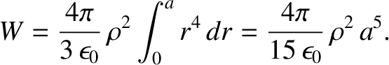 |
(2.89) |
This can also be written in terms of the total charge
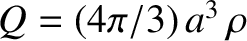 as
as
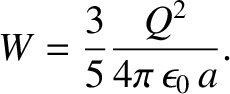 |
(2.90) |
Now that we have evaluated the potential energy of a spherical charge distribution
by the direct method, let us work it out using Equation (2.83). We shall assume that the
electric field is both radial and spherically symmetric, so that
 . Here, is a standard spherical polar coordinate. (See Section A.23.) Application of Gauss's law,
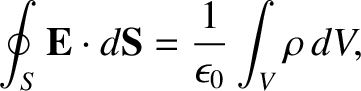 |
(2.91) |
where is a sphere of radius , centered on the origin, gives
 |
(2.92) |
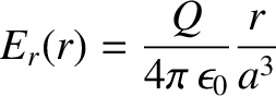
for  , and
, and
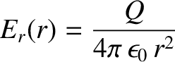 |
(2.93) |
for  . Equations (2.83), (2.92), and (2.93) yield
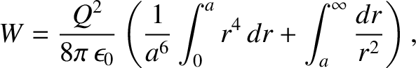 |
(2.94) |
which reduces to
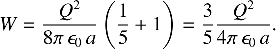 |
(2.95) |
Thus, Equation (2.83) gives the correct answer.
The reason that we have checked Equation (2.83) so carefully is that, on close inspection,
it is found to be
inconsistent with Equation (2.74), from which it was supposedly derived.
For instance, the energy given by Equation (2.83) is manifestly positive definite, whereas
the energy given by Equation (2.74) can be negative (it is certainly negative for
a collection of two point charges of opposite sign). The
inconsistency was introduced into our analysis when we replaced Equation (2.75) by
Equation (2.77). In Equation (2.75), the self-interaction of the th charge with its
own electric field is specifically excluded, whereas it is included in Equation (2.77). Thus,
the potential energies
(2.74) and (2.83) are different because in the former we start from
ready-made point charges, whereas in the latter we build up the whole
charge distribution from scratch. Hence, if we were to work out the
potential energy of a point charge distribution using Equation (2.83) then
we would obtain the energy (2.74) plus the energy required to assemble the
point charges. What is the energy required to assemble a point electric charge?
In fact, it is infinite. To see this, let us suppose, for the sake of argument, that
our point charges actually consist of electric charge uniformly distributed in small
spheres of radius  . According to Equation (2.90), the energy required to assemble the
th point charge is
. According to Equation (2.90), the energy required to assemble the
th point charge is
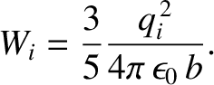 |
(2.96) |
We can think of this as the self-energy of the th charge.
Thus, we can write
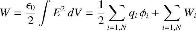 |
(2.97) |
which enables us to reconcile Equations (2.74) and (2.83). Unfortunately, if
our point charges really are point charges then
 , and the
self-energy of each charge becomes infinite. Thus, the potential
energies predicted by Equations (2.74) and (2.83) differ by an infinite amount.
What does this all mean? We have to conclude that the idea of locating electrostatic
potential energy in the electric field runs into conceptual difficulties in the presence of point electric charges. One way out of this dilemma would be to
say that elementary electric charges, such as protons and electrons, are not point objects, but instead have finite spatial extents. Regrettably, although protons have finite spatial extents (of about
, and the
self-energy of each charge becomes infinite. Thus, the potential
energies predicted by Equations (2.74) and (2.83) differ by an infinite amount.
What does this all mean? We have to conclude that the idea of locating electrostatic
potential energy in the electric field runs into conceptual difficulties in the presence of point electric charges. One way out of this dilemma would be to
say that elementary electric charges, such as protons and electrons, are not point objects, but instead have finite spatial extents. Regrettably, although protons have finite spatial extents (of about
 ), electrons really do seem to be point objects.