Electric Scalar Potential

We now have a problem. We can only write the electric field in terms of a scalar potential (i.e., ${\bf E} = -\nabla\phi$) provided that $\nabla\times{\bf E} = {\bf0}$. This follows because $\nabla\times \nabla\phi\equiv 0$. (See Section A.22.) However, we have just discovered that the curl of the electric field is non-zero in the presence of a changing magnetic field. In other words, ${\bf E}$ is not, in general, a conservative field. Does this mean that we have to abandon the concept of electric scalar potential? Fortunately, it does not. It is still possible to define a scalar potential that is physically meaningful.

Let us start from the field equation

$$\nabla\cdot {\bf B} = 0,$$ (2.293)

which is valid for both time-varying and constant magnetic fields. Because the magnetic field is solenoidal, we can write it as the curl of a vector potential:

$${\bf B} = \nabla\times{\bf A}.$$ (2.294)

[See Equation (2.251)]. This follows because $\nabla\cdot(\nabla\times{\bf A})\equiv 0$. (See Section A.22.) So, there is no problem with the vector potential in the presence of time-varying fields. Let us substitute Equation (2.294) into the field equation (2.286). We obtain

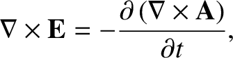$$\nabla\times{\bf E} = - \frac{\partial \,(\nabla\times{\bf A})}{\partial t},$$ (2.295)

which can be written

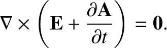$$\nabla\times\left( {\bf E} + \frac{\partial {\bf A} }{\partial t} \right) ={\bf0}.$$ (2.296)

Now, we know that a curl-free vector field can always be expressed as the gradient of a scalar potential (see Section A.22), so let us write

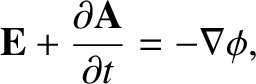$${\bf E} + \frac{\partial {\bf A} }{\partial t} = -\nabla\phi,$$ (2.297)

or

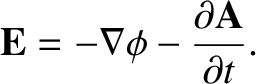$${\bf E} = - \nabla\phi - \frac{\partial {\bf A} }{\partial t}.$$ (2.298)

This equation implies that the electric scalar potential, $\phi$, only describes the conservative electric field generated by electric charges. The electric field induced by time-varying magnetic fields is non-conservative, and is described by the magnetic vector potential, ${\bf A}$.