Next: Inductance Up: Magnetic Induction Previous: Electric Scalar Potential
 and
and  fields unchanged in
Equations (2.299) and (2.300) is
where
fields unchanged in
Equations (2.299) and (2.300) is
where
 is a general scalar field known as the gauge field. A particular choice of the
gauge field is termed a choice of the gauge.
is a general scalar field known as the gauge field. A particular choice of the
gauge field is termed a choice of the gauge.
We are free to choose the gauge so as to make our equations as simple as possible. As before, the most sensible gauge for the scalar potential is to set it to zero at infinity:
   |
(2.303) |
 |
(2.304) |
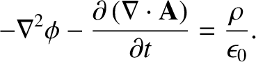
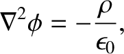
Equation (2.299) can be combined with the field equation [see Equation (2.54)]
 |
(2.305) |
 , the previous expression
reduces to
, the previous expression
reduces to
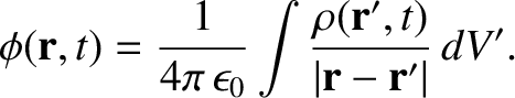
 |
(2.307) |
 then the potential at
  responds immediately.
However, special relativity forbid information from propagating faster than the speed of light in vacuum, because this
would violate causality. (See Section 3.2.10.) How can these two statements be reconciled? The crucial point is
that the scalar potential cannot be measured directly, it can only be inferred
from the electric field. In the time dependent case, there are two parts to the
electric field; that part that comes from the scalar potential, and that part
that comes from the vector potential. [See Equation (2.299).] So, if the scalar
potential in some region responds immediately to some distance rearrangement of charge density then
it does not necessarily follow that the electric field also has an immediate response.
What actually happens is that the change in the part of the
electric field that comes from
the scalar
potential is balanced by an equal and opposite change in the part that comes from the
vector potential, so that the overall electric field remains unchanged. This state
of affairs persists at least until sufficient time has elapsed for a light
signal to travel from the distant charges to the region in question.
Thus, causality is not violated, because it is the
electric field, and not the scalar potential, that carries physically accessible
information.
responds immediately.
However, special relativity forbid information from propagating faster than the speed of light in vacuum, because this
would violate causality. (See Section 3.2.10.) How can these two statements be reconciled? The crucial point is
that the scalar potential cannot be measured directly, it can only be inferred
from the electric field. In the time dependent case, there are two parts to the
electric field; that part that comes from the scalar potential, and that part
that comes from the vector potential. [See Equation (2.299).] So, if the scalar
potential in some region responds immediately to some distance rearrangement of charge density then
it does not necessarily follow that the electric field also has an immediate response.
What actually happens is that the change in the part of the
electric field that comes from
the scalar
potential is balanced by an equal and opposite change in the part that comes from the
vector potential, so that the overall electric field remains unchanged. This state
of affairs persists at least until sufficient time has elapsed for a light
signal to travel from the distant charges to the region in question.
Thus, causality is not violated, because it is the
electric field, and not the scalar potential, that carries physically accessible
information.
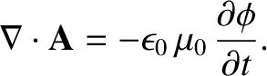
It is clear that the apparent action at a distance nature of Equation (2.308) is highly misleading. This suggests, very strongly, that the Coulomb gauge is not the optimum gauge in the time dependent case. A more sensible choice is the so-called Lorenz gauge:
Substituting the Lorenz gauge into Equation (2.306), we obtain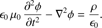 |
(2.310) |