We have already learned about the concepts of voltage, resistance, and capacitance. Let us now investigate the concept of inductance.
Electrical engineers like to reduce all pieces of electrical circuitry to an
equivalent circuit consisting of pure voltage sources,
pure inductors, pure capacitors, and pure resistors. Hence, once we understand inductors, we shall
be ready to apply the laws of electromagnetism to general electrical circuits.
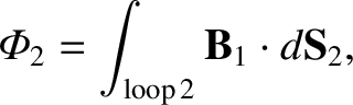
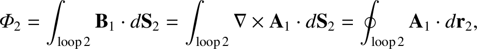
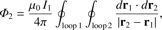
Consider two stationary loops of wire, labeled 1 and 2. See Figure 2.26. Let us run a steady current
 around the first loop to produce a magnetic field
  . Some of the field-lines
of will pass through the second loop. Let
. Some of the field-lines
of will pass through the second loop. Let
 be the flux
of through loop 2,
be the flux
of through loop 2,
 |
(2.311) |
where
 is a surface element of loop 2.
This flux is generally quite difficult to calculate exactly (unless the two loops
have a particularly simple geometry). However, we can infer from the Biot-Savart law [see Equation (2.226)],
is a surface element of loop 2.
This flux is generally quite difficult to calculate exactly (unless the two loops
have a particularly simple geometry). However, we can infer from the Biot-Savart law [see Equation (2.226)],
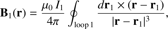 |
(2.312) |
that the magnitude of is proportional to the current .
Here,
 is a line element of loop 1 located at displacement
  .
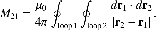
It follows that
the flux
must also be proportional to . Thus, we can write
.
It follows that
the flux
must also be proportional to . Thus, we can write
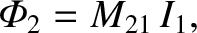 |
(2.313) |
where  is a constant of proportionality. This constant is termed
the mutual inductance of the two loops.
is a constant of proportionality. This constant is termed
the mutual inductance of the two loops.
Figure 2.26:
Two current-carrying loops.
|
|
Let us write the magnetic field in terms of a vector potential  , so that
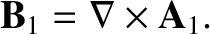 |
(2.314) |
It follows from the curl theorem (see Section A.22) that
 |
(2.315) |
where
 is a line element of loop 2.
However, we know that
is a line element of loop 2.
However, we know that
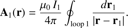 |
(2.316) |
The previous equation is just a special case of the more general result [see Equation (2.252)],
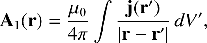 |
(2.317) |
for
 and
and
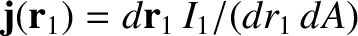
 , where
 is the cross-sectional area of loop 1. Thus,
 |
(2.318) |
where  is the position vector of the line element
of loop 2, which implies that
is the position vector of the line element
of loop 2, which implies that
 |
(2.319) |
In fact, mutual
inductances are rarely worked out using the previous formula, because it is usually
far too difficult. However, this formula, which is known as the Neumann formula, tells us two important things.
Firstly, the mutual inductance of two current loops is a purely geometric quantity,
having to do with the sizes, shapes, and relative orientations of the loops.
Secondly, the integral is unchanged if we switch the roles of loops 1 and 2.
In other words,
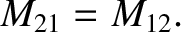 |
(2.320) |
Hence, we can drop the subscripts, and just call both of these quantities  .
This result implies that no matter what the shapes and
relative positions of the two loops, the magnetic flux through loop 2 when a
current
.
This result implies that no matter what the shapes and
relative positions of the two loops, the magnetic flux through loop 2 when a
current  runs around loop 1 is exactly the same as the flux through loop 1
when the same current runs around loop 2.
runs around loop 1 is exactly the same as the flux through loop 1
when the same current runs around loop 2.
We have seen that a current flowing around some wire loop, 1, generates a magnetic
flux linking some other loop, 2. However, flux is also generated through the
first loop. As before, the magnetic field, and, therefore, the flux,
 ,
is proportional to the current, so we can write
,
is proportional to the current, so we can write
 |
(2.321) |
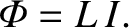
The constant of proportionality  is called the self inductance. Like
it only depends on the geometry of the loop.
is called the self inductance. Like
it only depends on the geometry of the loop.
The SI unit of inductance is the henry (H), which is equivalent to a volt-second
per ampere. The henry, like the farad, is a rather unwieldy unit, because
inductors in electrical circuits typically have a inductances of order a micro-henry.
![\includegraphics[height=2in]{Chapter03/loop.eps}](img1736.png)