Electromagnetic Waves
Let us demonstrate that Maxwell's equations possess
wave-like solutions that can propagate through a vacuum. These solutions are known
as electromagnetic waves. Let us start from Maxwell's equations
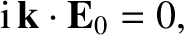
in free space (i.e., with no charges and no currents):
[See Equations (2.484)–(2.487).]
There is an easy way to show that the previous equations possess wave-like
solutions, and a hard way. The easy way is to assume that the solutions are
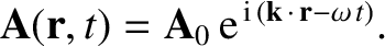
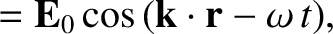
going to be wave-like beforehand. Specifically, let us search for
plane-wave solutions of the form:
Here,  and
and  are constant vectors,
  is known as
the wavevector, and
is known as
the wavevector, and  is the angular frequency of oscillation of the wave. The frequency
in hertz,
is the angular frequency of oscillation of the wave. The frequency
in hertz,  , is related to the angular frequency via
 ; this frequency is conventionally defined to be positive. The quantity
 is a phase difference between the electric and magnetic fields.
Actually, it is more convenient to write
where, by convention, the physical solution is the real part of the
previous equations. The phase difference is absorbed into the
constant vector by allowing it to become complex. Thus,
is a phase difference between the electric and magnetic fields.
Actually, it is more convenient to write
where, by convention, the physical solution is the real part of the
previous equations. The phase difference is absorbed into the
constant vector by allowing it to become complex. Thus,
 . In general,
the vector is also complex.
. In general,
the vector is also complex.
Now, assuming (without loss of generality) that is real, a wave maximum of the electric field satisfies
 |
(2.512) |
where  is an integer. The solution to
this equation is a set of equally-spaced parallel planes
(one plane for each possible value of ), whose normals are parallel
to the wavevector , and
that propagate in the direction of with phase velocity
is an integer. The solution to
this equation is a set of equally-spaced parallel planes
(one plane for each possible value of ), whose normals are parallel
to the wavevector , and
that propagate in the direction of with phase velocity
 |
(2.513) |
The spacing between adjacent planes (i.e., the wavelength) is given by
 |
(2.514) |
See Figure 2.40.
Figure 2.40:
Wavefronts associated with a plane wave.
|
|
Consider a general plane-wave vector field
 |
(2.515) |
What is the divergence of  ? This is easy to evaluate. We have
(See Section A.20.)
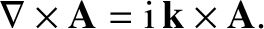
How about the curl of ? This is slightly more difficult. We have
? This is easy to evaluate. We have
(See Section A.20.)
How about the curl of ? This is slightly more difficult. We have
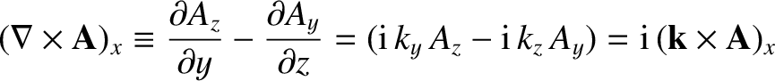 |
(2.517) |
 |
(2.518) |
Hence, it is apparent that vector field operations on a plane-wave vector field are equivalent to
replacing the  operator with
 . Of course, the
 operator can be replaced by
 .
.
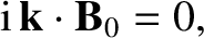
The first Maxwell equation, (2.504), reduces to
 |
(2.519) |
using the assumed electric and magnetic fields, (2.510) and (2.511), and
Equation (2.516). Thus, the electric field is perpendicular to the direction
of propagation of the wave. (See Section A.6.) Likewise, the second Maxwell equation, (2.505), gives
 |
(2.520) |
implying that the magnetic field is also perpendicular to the direction of
propagation. Clearly, the wave-like solutions of Maxwell's equation
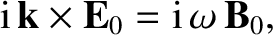
are a type of transverse wave. The third Maxwell equation, (2.506), yields
 |
(2.521) |
where use has been made of Equation (2.518). Forming the scalar product of this equation with
gives
 |
(2.522) |
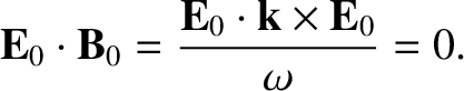
Thus, the electric and magnetic fields are mutually perpendicular. (See Sections A.6 and A.10.) Forming the scalar product of
Equation (2.521) with yields
 |
(2.523) |
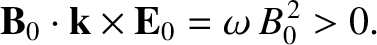
Thus, the vectors , , and are mutually
perpendicular, and form a right-handed set. (See Section A.10.) The final Maxwell equation, (2.507),
gives
 |
(2.524) |
Combining this equation with Equation (2.521) yields
 |
(2.525) |
or
 |
(2.526) |
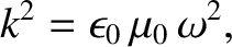
where use has been made of Equation (2.519). (See Section A.11.) However, we know, from Equation (2.513), that
the phase velocity,  , of the wave is related to the magnitude of the wavevector and the
angular wave frequency via
, of the wave is related to the magnitude of the wavevector and the
angular wave frequency via
 . Thus, we obtain
 |
(2.527) |
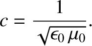
We have found transverse plane-wave solutions of the free-space Maxwell equations
propagating at some phase velocity , that is given by a combination of
 and
and
 , and is, thus, the same for all frequencies and wavelengths. The constants
and
are easily measurable. The former is related to the
force acting between stationary electric charges, and the latter to the force acting between steady electric currents.
Both of these constants were fairly well known in Maxwell's time. Maxwell,
incidentally, was the first person to look for wave-like solutions of
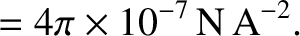
his equations, and, thus, to derive Equation (2.527). The modern values of
and are
, and is, thus, the same for all frequencies and wavelengths. The constants
and
are easily measurable. The former is related to the
force acting between stationary electric charges, and the latter to the force acting between steady electric currents.
Both of these constants were fairly well known in Maxwell's time. Maxwell,
incidentally, was the first person to look for wave-like solutions of
his equations, and, thus, to derive Equation (2.527). The modern values of
and are
Let us use these values to find the phase velocity of electromagnetic
waves. We obtain
 |
(2.530) |
Of course, we immediately recognize this as the speed of light in vacuum. Maxwell also made
this connection back in the 1870's. He conjectured that light, whose nature had
previously been unknown, was a form of electromagnetic radiation. This was
a remarkable
prediction. After all, Maxwell's equations were derived from the results of bench-top
laboratory experiments involving charges, batteries, coils, and currents, that apparently
had nothing
whatsoever to do with light.
Maxwell was able to make another remarkable prediction. The wavelength of
light was well-known in the late nineteenth century from studies of diffraction
through slits, et cetera.
Visible light actually occupies a surprisingly
narrow wavelength range. The shortest wavelength blue light that is visible to the typical human eye
has a wavelength of
 microns (one micron is
  meters).
The longest wavelength red light that is visible has
a wavelength of
meters).
The longest wavelength red light that is visible has
a wavelength of
 microns. However, there is nothing in our analysis that suggests that
this particular range of wavelengths is special. Electromagnetic waves
can have any wavelength.
Maxwell concluded that visible light was a small part of a vast spectrum of
previously undiscovered
types of electromagnetic radiation. Since Maxwell's time, virtually all of the
non-visible parts of the electromagnetic spectrum have been observed.
microns. However, there is nothing in our analysis that suggests that
this particular range of wavelengths is special. Electromagnetic waves
can have any wavelength.
Maxwell concluded that visible light was a small part of a vast spectrum of
previously undiscovered
types of electromagnetic radiation. Since Maxwell's time, virtually all of the
non-visible parts of the electromagnetic spectrum have been observed.
Table 1 gives a brief guide to the electromagnetic spectrum.
Electromagnetic waves are of particular importance to us because they
are our main source of information regarding the universe around us.
Radio waves and microwaves (which are comparatively
hard to scatter) have provided much of
our knowledge about the center of our own galaxy. This is completely unobservable
in visible light, which is strongly scattered by interstellar gas and dust
lying in the galactic plane.
For the same reason, the spiral arms of our galaxy can only be mapped out using radio waves.
Infrared radiation is useful for detecting
protostars, which are not yet hot enough to emit visible radiation.
Of course, visible radiation is still the mainstay of astronomy.
Satellite-based ultraviolet observations have yielded invaluable insights into
the structure and distribution of distant galaxies. Finally, X-ray and  -ray
astronomy usually concentrates on exotic objects, such as pulsars
and supernova remnants.
-ray
astronomy usually concentrates on exotic objects, such as pulsars
and supernova remnants.
Table 2.1:
The electromagnetic spectrum
| Radiation type |
Wavelength range ( ) ) |
| Gamma Rays |
 |
| X-Rays |
 – – |
| Ultraviolet |
– |
| Visible |
– |
| Infrared |
– |
| Microwave |
– |
| TV-FM |
– |
| Radio |
 |
|
Equations (2.519), (2.521), and the relation
, imply that
 |
(2.531) |
Thus, the magnetic field associated with an electromagnetic wave is smaller
in magnitude than the electric field by a factor . Consider
an electrically charged particle interacting with an electromagnetic wave. The force exerted on the
particle is given by the Lorentz force law,
 |
(2.532) |
(See Section 2.2.4.)
The ratio of the electric and magnetic forces is
 |
(2.533) |
So, unless the particle is moving close to the speed of light (i.e., unless the particle is relativistic), the electric force greatly exceeds the
magnetic force. Clearly, in most terrestrial situations, electromagnetic waves are
an essentially electrical phenomenon (as far as their interaction with matter is concerned).
For this reason, electromagnetic waves are usually characterized by their wavevector,
(which specifies the direction of propagation and the wavelength), and
the plane of polarization (i.e., the plane of oscillation) of the associated electric
field. For a given wavevector, , the electric field can have any direction in
the plane normal to . [See Equation (2.519).] However, there are only two independent
directions in a plane (i.e., we can only define two linearly independent
vectors in a plane). This implies that there are only two independent polarizations
of an electromagnetic wave, once its direction of propagation is
specified.
But, how do electromagnetic waves propagate through a vacuum? After
all, most types of wave require a medium before they can propagate
(e.g., sound waves require air). The answer to this question
is evident from Equations (2.506) and (2.507). According to these
equations, the time variation of the electric component of the
wave induces the magnetic component, and the time variation of
the magnetic component induces the electric component. In other words, electromagnetic
waves are self-sustaining, and, therefore, require no medium through which
to propagate.
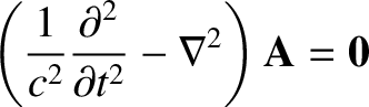
Let us now search for the wave-like solutions of Maxwell's equations in free-space the hard way.
Suppose that we take the curl of the fourth Maxwell equation, (2.507). We obtain
 |
(2.534) |
[See Equation (A.187).]
Here, we have made use of the fact that
 , according to the second Maxwell equation, (2.505). The third Maxwell equation,
(2.506), yields
, according to the second Maxwell equation, (2.505). The third Maxwell equation,
(2.506), yields
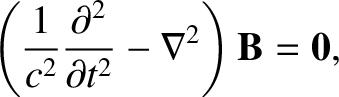 |
(2.535) |
where use has been made of Equation (2.530). A similar equation can obtained for the electric field
by taking the curl of Equation (2.506):
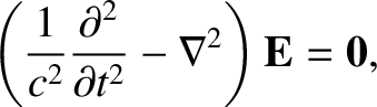 |
(2.536) |
Figure 2.41:
An arbitrary wave-pulse.
|
|
We have found that electric and magnetic fields both satisfy equations of the
form
 |
(2.537) |
in free space. As is easily verified, the
most general solution to this equation is
where  is a unit vector, and
  ,
,  , and
, and  are arbitrary
one-dimensional
scalar functions. Looking along the direction of , so that
are arbitrary
one-dimensional
scalar functions. Looking along the direction of , so that
 ,
we find that
The
,
we find that
The  -component of this solution is shown schematically in Figure 2.41. The solution clearly propagates along the
 -axis,
at the speed , without changing shape.
If we look along a direction that is perpendicular to then
-axis,
at the speed , without changing shape.
If we look along a direction that is perpendicular to then
 , and there is no propagation.
Thus, the components
of
are arbitrarily-shaped pulses that propagate, without changing shape, along
the direction of
with speed .
These pulses can be related to the sinusoidal plane-wave solutions which we found earlier
by Fourier transformation; that is,
, and there is no propagation.
Thus, the components
of
are arbitrarily-shaped pulses that propagate, without changing shape, along
the direction of
with speed .
These pulses can be related to the sinusoidal plane-wave solutions which we found earlier
by Fourier transformation; that is,
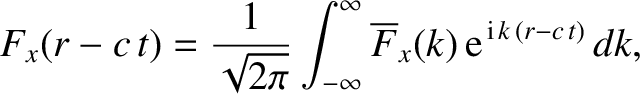 |
(2.544) |
where
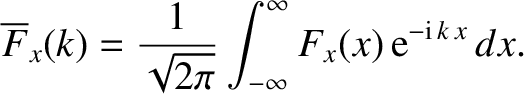 |
(2.545) |
(See Section 4.2.4.)
Thus, any arbitrary-shaped pulse propagating in the direction of
with speed can be broken down into a superposition of sinusoidal oscillations of different wavevectors,
 , propagating
in the same direction with the same speed.
, propagating
in the same direction with the same speed.


![\includegraphics[height=2.5in]{Chapter03/fig4_3.eps}](img2113.png)


![\includegraphics[height=2.5in]{Chapter03/fig4_4.eps}](img2150.png)