Potential Formulation of Maxwell's Equations

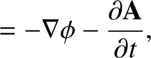
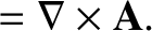
We saw in Section 2.3.2 that the second and third Maxwell equations, (2.485) and (2.486), are automatically satisfied if we write the electric and magnetic fields in terms of scalar and vector potentials; that is,

$${\bf E} = - \nabla\phi - \frac{\partial {\bf A}}{\partial t},$$ (2.495)

$${\bf B} = \nabla\times{\bf A}.$$ (2.496)

As was discussed in Section 2.3.3, this prescription is not unique, but we can make it unique by adopting the following conventions:

$$\phi({\bf r}) \rightarrow 0 \mbox{\hspace{0.5cm}as~~~$\vert{\bf r}\vert \rightarrow \infty$} ,$$ (2.497)

$$\nabla\cdot {\bf A} = -\epsilon_0\, \mu_0 \,\frac{\partial \phi}{\partial t}.$$ (2.498)

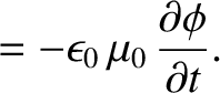
The previous equation is known as the Lorenz gauge.

The previous equation can be combined with Equation (2.495) and the first Maxwell equation, (2.484), to give

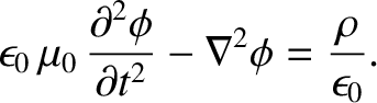$$\epsilon_0\,\mu_0\,\frac{\partial^2\phi}{\partial t^2} - \nabla^2\phi = \frac{\rho} {\epsilon_0}.$$ (2.499)

Let us now consider the fourth Maxwell equation, (2.487). Substitution of Equations (2.495) and (2.496) into this equation yields

$$\nabla\times\nabla\times {\bf A} \equiv \nabla(\nabla\cdot{\bf A}... ...\phi}{\partial t} - \epsilon_0\,\mu_0\, \frac{\partial^2 {\bf A}}{\partial t^2}$$ (2.500)

(see Section A.24), or

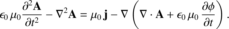$$\epsilon_0 \,\mu_0 \frac{\partial^2 {\bf A}}{\partial t^2} - \nab... ...nabla\cdot{\bf A} +\epsilon_0\,\mu_0\, \frac{\partial\phi} {\partial t}\right).$$ (2.501)

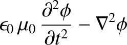
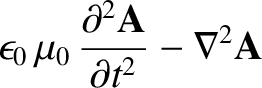
We can now see quite clearly where the Lorenz gauge, (2.498), comes from. The previous equation is, in general, very complicated, because it involves both the vector and scalar potentials. However, if we adopt the Lorenz gauge then the last term on the right-hand side becomes zero, and the equation simplifies considerably, and ends up only involving the vector potential. Thus, we find that Maxwell's equations reduce to the following equations:

$$\epsilon_0\,\mu_0\,\frac{\partial^2\phi}{\partial t^2} - \nabla^2\phi = \frac{\rho}{\epsilon_0},$$ (2.502)

$$\epsilon_0\,\mu_0\,\frac{\partial^2{\bf A} }{\partial t^2} - \nabla^2{\bf A} = \mu_0 \,{\bf j}.$$ (2.503)

Of course, this is the same (scalar) equation written four times over. In a non-time-varying situation (i.e., $\partial/\partial t=0$), the equation in question reduces to Poisson's equation (see Section 2.1.9), which we know how to solve. With the $\partial^2/\partial t^2$ terms included, the equation becomes a slightly more complicated equation (in fact, it is an inhomogeneous three-dimensional wave equation).