Ampère's Circuital Law

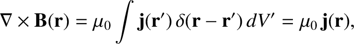
According to Equation (2.251),

$$\nabla\times {\bf B} = \nabla\times(\nabla\times {\bf A})\equiv \nabla\,(\nabla\cdot{\bf A})- \nabla^{\,2}{\bf A},$$ (2.266)

where use has been made of Equation (A.187). However, Equation (2.262) indicates that $\nabla\cdot {\bf A}=0$ for a steady current distribution. Hence, the previous equation simplifies to give

$$\nabla\times {\bf B} =- \nabla^{\,2}{\bf A}.$$ (2.267)

The previous equation can be combined with Equation (2.252) to give

$$\nabla\times{\bf B}({\bf r})= -\frac{\mu_0}{4\pi}\int {\bf j}({\bf r}')\,\nabla^2\!\left(\frac{1}{\vert{\bf r}-{\bf r}'\vert}\right)dV'.$$ (2.268)

However, according to Equation (2.56),

$$\nabla^2\!\left(\frac{1}{\vert{\bf r} - {\bf r}'\vert}\right)= -4\pi\,\delta({\bf r} -{\bf r}'),$$ (2.269)

so we obtain

$$\nabla\times {\bf B}({\bf r}) = \mu_0\int {\bf j}({\bf r}')\,\delta({\bf r}-{\bf r}')\,dV' =\mu_0\,{\bf j}({\bf r}),$$ (2.270)

where use has been made of Equation (2.47).

The previous equation can be written

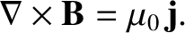$$\nabla\times {\bf B}= \mu_0\,{\bf j}.$$ (2.271)

Let us calculate the flux of $\mu_0\,{\bf j}$ through some surface $S$, bounded by a loop $C$. Making use of the previous field equation, as well as the curl theorem (see Section A.22), we obtain

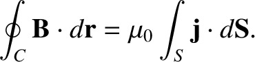$$\oint_C {\bf B}\cdot d{\bf r} = \mu_0\int_S{\bf j}\cdot d{\bf S}.$$ (2.272)

In other words, the line integral of the magnetic field around some loop $C$ is equal to $\mu_0$ multiplied by the net electric current flowing across some surface, $S$, attached to the loop. This result is known as Ampère's circuital law. Note that because the current density associated with a steady current pattern is divergence free [see Equation (2.261)], the net current flowing across any surface attached to $C$ is the same. (See Section A.20.) Of course, when performing the line integral we have to choose an arbitrary sense of circulation around the loop. Once we have done this, any currents that the loop circles in an counter-clockwise direction (looking against the direction of the current) count as positive currents, whereas any currents that the loop circles in a clockwise direction (looking against the direction of the current) count as negative currents.

Let us apply Ampère's circuital law to the trivial case of a circular loop of radius $r$ that lies in the plane perpendicular to a long straight wire, carrying a current $I$, that passes though its center. By symmetry, we expect the magnetic field to be of the form 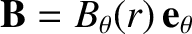${\bf B}= B_\theta(r)\,{\bf e}_\theta$, where $r$, $\theta$, $z$ are right-handed cylindrical polar coordinates defined such that the wire runs along the $z$-axis. (See Section A.23.) If the chosen sense of circulation around the loop is in the direction of increasing $\theta$ then $I$ counts as a positive current. Thus, Equation (2.272) yields

$$2\pi\,r\,B_\theta(r) = \mu_0\,I,$$ (2.273)

or

$$B_\theta = \frac{\mu_0\,I}{2\pi\,r},$$ (2.274)

which is equivalent to Equation (2.206).

Figure 2.23: An example use of Ampère's circuital law.

As another example of the use of Ampère's circuital law, let us calculate the magnetic field generated by a cylindrical current annulus of inner radius $a$, and outer radius $b$, co-axial with the $z$-axis, and carrying a uniformly distributed $z$-directed current $I$. By symmetry, and also by analogy with the magnetic field generated by a straight wire, we expect the current distribution to generate a magnetic field of the form ${\bf B}= B_\theta(r)\,{\bf e}_\theta$, where $r$, $\theta$, $z$ are right-handed cylindrical polar coordinates. (See Section A.23.) Let us apply Ampère's circuital law to an imaginary circular loop in the $x$-$y$ plane, of radius $r$, centered on the $z$-axis. See Figure 2.23. Such a loop is generally known as an Ampèrian loop. As before, if the chosen sense of circulation around the loop is in the direction of increasing $\theta$ then $I$ counts as a positive current. According to Ampère's circuital law, the line integral of the magnetic field around the loop is equal to the current passing through the plane of the loop, multiplied by $\mu_0$. The line integral is easy to calculate because the magnetic field is everywhere tangential to the loop. We obtain

$$2\pi\,r\,B_\theta(r) = \mu_0\,I(r),$$

where $I(r)$ is the current that passes through an Ampèrian loop of radius $r$. Simple arguments involving proportion reveal that

$$I(r) = \left\{ \begin{array}{lcl} 0&\mbox{\hspace{1cm}}&r<a\\... ...2)\right] I&&a\leq r\leq b\\ [0.5ex] I&&b<r \end{array}\right..$$ (2.275)

Hence,

$$B_\theta(r) = \left\{ \begin{array}{lcl} 0&\mbox{\hspace{1cm}... ...q r\leq b\\ [0.5ex] \mu_0\,I/(2\pi\,r)&&b<r \end{array}\right..$$ (2.276)