Next: Capacitors Up: Electrostatic Fields Previous: Ohm's Law
 ,
acting around each loop (unless the conductor is a
superconductor, with
,
acting around each loop (unless the conductor is a
superconductor, with  ). However, we know that in a steady state
 |
(2.123) |
 . [See Equation (2.24).] This proves that a steady-state emf acting around
a closed loop inside a conductor is impossible. The only other alternative is
everywhere inside the conductor. It immediately follows from the field equation
. [See Equation (2.24).] This proves that a steady-state emf acting around
a closed loop inside a conductor is impossible. The only other alternative is
everywhere inside the conductor. It immediately follows from the field equation
 [see Equation (2.54)]
that
[see Equation (2.54)]
that
 |
(2.125) |
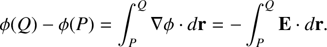
Now, the difference in scalar potential between
two points  and
and  is simply
and both lie inside the same conductor
then it is clear from Equations (2.124) and (2.126) that the potential difference between and
is zero. This is true no matter where and are situated inside the
conductor, so we conclude that the scalar potential must be
uniform inside a conductor.
One corollary of this fact is that the surface of a conductor is
an equipotential (i.e.,  constant) surface.
We have demonstrated that the electric field inside a conductor is zero. We can also demonstrate that the field within an empty cavity lying inside a conductor is
zero, provided that there are no charges within the cavity. Let  be the cavity in question, and let
  be its bounding
surface. Because there are no electric charges within the cavity, the electric potential,
be its bounding
surface. Because there are no electric charges within the cavity, the electric potential,  , inside the cavity
satisfies
, inside the cavity
satisfies
corresponds to the inner surface of the conductor that surrounds the
cavity, is an equipotential surface. In other words, the electric potential on takes a constant value,  (say).
So, we need to solve a simplified version of Poisson's equation, (2.127), throughout , subject to the
boundary condition that
(say).
So, we need to solve a simplified version of Poisson's equation, (2.127), throughout , subject to the
boundary condition that
 on . One obvious solution to this problem is
throughout
and on . However, we showed in Section 2.1.10 that the solutions to Poisson's equation in a volume
surrounded by a surface on which the potential is specified are unique. Thus,
throughout
and on is the only solution to the problem. It follows that the electric field
on . One obvious solution to this problem is
throughout
and on . However, we showed in Section 2.1.10 that the solutions to Poisson's equation in a volume
surrounded by a surface on which the potential is specified are unique. Thus,
throughout
and on is the only solution to the problem. It follows that the electric field
 is
zero throughout the cavity. [See Equation (2.17).]
is
zero throughout the cavity. [See Equation (2.17).]
We have shown that if a charge-free cavity is completely enclosed by a conductor then no stationary distribution of charges outside the conductor can ever produce any electric fields inside the cavity. It follows that we can shield a sensitive piece of electrical equipment from stray external electric fields by placing it inside a metal can. In fact, a wire mesh cage will do, as long as the mesh spacing is not too wide. Such a cage is known as a Faraday cage.
Consider a small region lying on the surface of a conductor. Suppose that
the local surface electric charge density is  , and that the electric field just outside
the conductor is
, and that the electric field just outside
the conductor is  . Note that this field must be directed normal
to the surface of the conductor. Any parallel component would be shorted out
by surface currents. Another way of saying this is that the surface of a conductor
is an equipotential. We know that
. Note that this field must be directed normal
to the surface of the conductor. Any parallel component would be shorted out
by surface currents. Another way of saying this is that the surface of a conductor
is an equipotential. We know that
 is always perpendicular to
an equipotential (see Section A.18), so
[see Equation (2.17)] must be locally perpendicular
to a conducting surface. Let us use Gauss's law [see Equation (2.58)],
is always perpendicular to
an equipotential (see Section A.18), so
[see Equation (2.17)] must be locally perpendicular
to a conducting surface. Let us use Gauss's law [see Equation (2.58)],
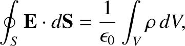 |
(2.128) |
is a so-called Gaussian pill-box. See Figure 2.5. A Gaussian pill-box is a volume of space whose shape is similar to an old-fashioned pill-box (or a modern pizza box).
Let the two flat ends of the pill-box be aligned parallel to the surface of the conductor,
with the surface running between them, and let the comparatively short sides be perpendicular to the
surface.
It is clear that is parallel to the sides of the box, so the sides
make no contribution to the surface integral. The end of the box that lies
inside the conductor also makes no contribution,
because
 inside a conductor. Thus, the only non-zero contribution to the
surface integral comes from the end lying in free space. This contribution
is simply
inside a conductor. Thus, the only non-zero contribution to the
surface integral comes from the end lying in free space. This contribution
is simply
 , where
  denotes an outward pointing (from the
conductor) normal
electric field, and
denotes an outward pointing (from the
conductor) normal
electric field, and  is the cross-sectional area of the box.
The charge enclosed
by the box is simply
is the cross-sectional area of the box.
The charge enclosed
by the box is simply  , from the definition of a surface charge density.
Thus, Gauss's law yields
as the relationship between the normal electric field immediately outside a conductor
and the surface charge density.
, from the definition of a surface charge density.
Thus, Gauss's law yields
as the relationship between the normal electric field immediately outside a conductor
and the surface charge density.
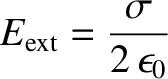
Let us look at the electric field generated by a sheet charge distribution
a little more carefully. Suppose that the charge per unit area is .
By symmetry, we expect the field generated below the sheet to be the mirror image
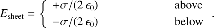
of that above the sheet (at least, locally). Thus, if apply Gauss's law to
a pill-box of cross-sectional area , as shown in Figure 2.6, then the
two ends both contribute
 to the surface integral, where
 is the normal
electric field generated above and below the sheet. The charge enclosed
by the pill-box is just . Thus, Gauss's law yields
a symmetric electric field
is the normal
electric field generated above and below the sheet. The charge enclosed
by the pill-box is just . Thus, Gauss's law yields
a symmetric electric field
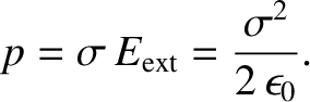
Making use of Equations (2.131) and (2.133), the electrostatic pressure acting at the surface of a conductor can also be written
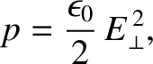 |
(2.134) |
is the electric field-strength immediately above the surface of the conductor.
Note that, according to the previous formula, the electrostatic pressure is equivalent
to the energy density of the electric field immediately outside the conductor. [See Equation (2.84).]
This is not a coincidence. Suppose that the conductor expands normally by an average
distance  , due to the electrostatic pressure. The electric field is excluded
from the region into which the conductor expands. The volume of this region
is
, due to the electrostatic pressure. The electric field is excluded
from the region into which the conductor expands. The volume of this region
is
 , where is the surface area of the conductor. Thus, the energy
of the electric field decreases by an amount
, where is the surface area of the conductor. Thus, the energy
of the electric field decreases by an amount
 ,
where
,
where  is the energy density of the field. This decrease in energy can be
ascribed to the work that the field does on the conductor in order to make it expand.
This work is
is the energy density of the field. This decrease in energy can be
ascribed to the work that the field does on the conductor in order to make it expand.
This work is
 , where
  is the force per unit area that the field exerts
on the conductor. Thus,
is the force per unit area that the field exerts
on the conductor. Thus,  , from energy conservation, giving
 |
(2.135) |
![\includegraphics[height=2.5in]{Chapter03/fig5_2.eps}](img1350.png)
![\begin{displaymath}E_{\rm total}= \left\{
\begin{array}{lll}
+\sigma/\epsilon_0&...
... [0.5ex]
0&\mbox{\hspace{2cm}}&\mbox{below}
\end{array}\right.,\end{displaymath}](img1355.png)
![\includegraphics[height=2.25in]{Chapter03/fig5_3.eps}](img1357.png)