Next: Method of Images Up: Electrostatic Fields Previous: Ideal Conductors
 volts per meter. This
phenomenon, which is known as breakdown, is associated with the formation
of sparks. The most well-known example of the breakdown of
air is during a lightning
strike. Thus, a good charge-storing device is one that holds a relatively large amount
of charge, but only generates relatively small external electric fields (so as to avoid breakdown). Such a device is called
a capacitor.
volts per meter. This
phenomenon, which is known as breakdown, is associated with the formation
of sparks. The most well-known example of the breakdown of
air is during a lightning
strike. Thus, a good charge-storing device is one that holds a relatively large amount
of charge, but only generates relatively small external electric fields (so as to avoid breakdown). Such a device is called
a capacitor.
Consider two thin, parallel, conducting
plates of cross-sectional area  that are separated by
a small distance
that are separated by
a small distance  (i.e.,
 ). Suppose that each plate
carries an equal and opposite charge
). Suppose that each plate
carries an equal and opposite charge  (where
  ). We expect this charge to
spread evenly over the plates to give an effective sheet charge density
). We expect this charge to
spread evenly over the plates to give an effective sheet charge density
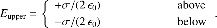
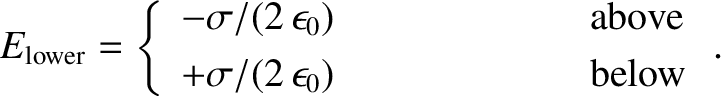
 on each plate. Suppose that the upper plate carries a
positive charge and that the lower carries a negative charge. According to
Equation (2.130), the field generated by the upper plate is normal to the plate and
of magnitude
on each plate. Suppose that the upper plate carries a
positive charge and that the lower carries a negative charge. According to
Equation (2.130), the field generated by the upper plate is normal to the plate and
of magnitude
 |
(2.136) |
 |
(2.137) |
![\begin{displaymath}E_\perp =\left\{
\begin{array}{lcl}
\sigma /\epsilon_0&\mbox{...
...ex]
0& \mbox{\hspace{2cm}}&\mbox{otherwise}
\end{array}\right..\end{displaymath}](img1372.png) |
(2.138) |
 |
(2.139) |
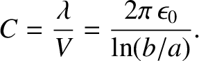
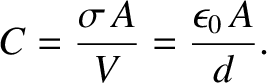
It is conventional to measure the capacity of a conductor, or set of conductors,
to store electric charge, but generate small external electric fields, in terms of a parameter
called capacitance. This parameter is
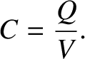
usually denoted  . The capacitance of a charge storing
device is simply the ratio of the charge stored to the potential difference
generated by this charge:
. The capacitance of a charge storing
device is simply the ratio of the charge stored to the potential difference
generated by this charge:
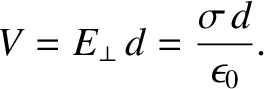
For a parallel plate capacitor, we have
Note that the capacitance only depends on geometric quantities, such as the area and spacing of the plates. This is a consequence of the superposability of electric fields. If we double the charge on a set of conductors then we double the electric fields generated around them, and we, therefore, double the potential difference between the conductors. Thus, the potential difference between the conductors is always directly proportional to the charge on the conductors. Moreover, the constant of proportionality (the inverse of the capacitance) can only depend on geometry.
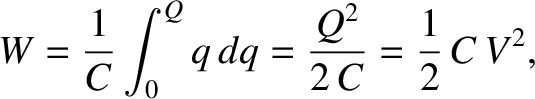
Suppose that the charge on each plate of a parallel plate capacitor is built up gradually by transferring
small amounts of charge from one plate to another. If the
instantaneous charge on the plates is  , and an infinitesimal amount of
positive
charge
, and an infinitesimal amount of
positive
charge  is transferred from the negatively charged to the positively
charge plate, then the work done is
is transferred from the negatively charged to the positively
charge plate, then the work done is
 ,
where
,
where  is the instantaneous
voltage difference between the plates. (See Section 2.1.5.) Note that the voltage difference is such
that it opposes any increase in the charge on either plate.
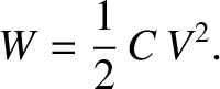
The total work done in charging the capacitor
is
is the instantaneous
voltage difference between the plates. (See Section 2.1.5.) Note that the voltage difference is such
that it opposes any increase in the charge on either plate.
The total work done in charging the capacitor
is
 |
(2.143) |
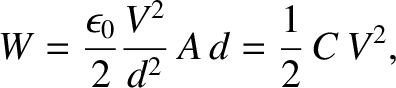
The energy of
a charged parallel
plate
capacitor is actually stored in the electric field generated between the plates. This field
is of approximately constant magnitude
 , and occupies a
region of volume
, and occupies a
region of volume  . Thus, given the energy density of an electric
field,
. Thus, given the energy density of an electric
field,
 [see Equation (2.84)], the energy stored in the
electric field is
[see Equation (2.84)], the energy stored in the
electric field is
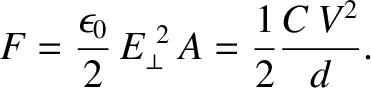
The idea, that we discussed in the previous section, that an electric field exerts a negative
pressure
 on conductors immediately suggests that
the two plates in a parallel plate capacitor attract one another with a
mutual force
on conductors immediately suggests that
the two plates in a parallel plate capacitor attract one another with a
mutual force
It is not actually necessary to have two oppositely charged conductors
in order to make a capacitor.
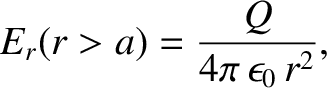
Consider an isolated
conducting sphere of radius  , centered on the origin, that
carries an electric charge
, centered on the origin, that
carries an electric charge  . The spherically symmetric, radial electric field generated outside the sphere is
given by
. The spherically symmetric, radial electric field generated outside the sphere is
given by
 |
(2.147) |
 is a spherical polar coordinate. (See Section A.23.)
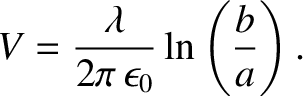
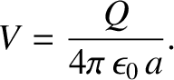
It follows that the potential difference between the sphere and infinity—or, more realistically,
some large, relatively distant reservoir of charge such as the Earth—is
Thus, the capacitance of the sphere is
is a spherical polar coordinate. (See Section A.23.)
It follows that the potential difference between the sphere and infinity—or, more realistically,
some large, relatively distant reservoir of charge such as the Earth—is
Thus, the capacitance of the sphere is
 |
(2.149) |
is again given by
 . It can easily be demonstrated that this is equivalent to
the energy contained in the electric field surrounding the capacitor.
. It can easily be demonstrated that this is equivalent to
the energy contained in the electric field surrounding the capacitor.
Suppose that we have two spheres of radii and  , respectively, that are
connected by a long electric wire. See Figure 2.8. The wire allows electric charge to move back and forth between
the spheres until they reach the same potential (with respect to infinity).
Let
, respectively, that are
connected by a long electric wire. See Figure 2.8. The wire allows electric charge to move back and forth between
the spheres until they reach the same potential (with respect to infinity).
Let  be the charge on the first sphere, and
  the charge on the
second sphere.
Of course, the total charge
the charge on the
second sphere.
Of course, the total charge
 carried by the two spheres is a conserved
quantity. It follows from Equation (2.148) that if the spheres are at the same potential then
carried by the two spheres is a conserved
quantity. It follows from Equation (2.148) that if the spheres are at the same potential then
 |
 |
(2.150) |
 |
 |
(2.151) |
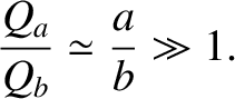
 —then
the large sphere grabs most of the charge; that is,
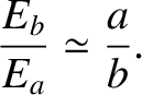
The ratio of the electric fields generated just above the surfaces of the two
spheres follows from Equations (2.146) and (2.152):
Note that if then the field just above the smaller sphere
is far larger than that above the larger sphere.
Equation (2.153) is a simple example of a far more general rule; namely,
the electric field directly above some point on the
surface of a conductor is inversely proportional to
the local radius of curvature of the surface.
—then
the large sphere grabs most of the charge; that is,
The ratio of the electric fields generated just above the surfaces of the two
spheres follows from Equations (2.146) and (2.152):
Note that if then the field just above the smaller sphere
is far larger than that above the larger sphere.
Equation (2.153) is a simple example of a far more general rule; namely,
the electric field directly above some point on the
surface of a conductor is inversely proportional to
the local radius of curvature of the surface.
It is clear that if we wish to store significant amounts of charge on a conductor then the surface of the conductor must be made as smooth as possible. Any sharp spikes on the surface will inevitably have comparatively small radii of curvature. Intense local electric fields are thus generated around such spikes. These fields can easily exceed the critical field for the breakdown of air, leading to sparking and the eventual loss of the charge on the conductor. Sparking can also be very destructive, because the associated electric currents flow through very localized regions, giving rise to intense ohmic heating.
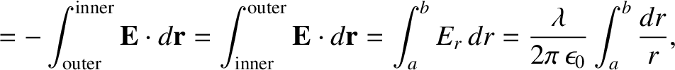
As a final example, consider two co-axial
conducting cylinders of radii and
, where  . Suppose that the charge per unit length carried by the
outer and inner cylinders is
. Suppose that the charge per unit length carried by the
outer and inner cylinders is  and
and  , respectively. We can safely
assume that
, respectively. We can safely
assume that
 , by symmetry (adopting
standard cylindrical polar coordinates). (See Section A.23.) Let us apply
Gauss's law (see Section 2.4) to a cylindrical surface of radius , co-axial with the conductors, and
of length
, by symmetry (adopting
standard cylindrical polar coordinates). (See Section A.23.) Let us apply
Gauss's law (see Section 2.4) to a cylindrical surface of radius , co-axial with the conductors, and
of length  . For
. For  , we find that
 |
(2.154) |
 |
(2.155) |
. It is fairly obvious that  if is not in the range
to . The potential difference between the inner and outer cylinders is [see Equation (2.17)]
if is not in the range
to . The potential difference between the inner and outer cylinders is [see Equation (2.17)]
 |
 |
(2.156) |
 |
(2.157) |
 |
(2.158) |
![\includegraphics[height=1.75in]{Chapter03/fig5_5.eps}](img1374.png)
![\includegraphics[height=1.5in]{Chapter03/fig5_6.eps}](img1402.png)