Method of Images
Suppose that a point electric charge  is located a distance
  from an infinite,
grounded (i.e., held at zero potential), conducting plate. See Figure 2.9. Let the plate lie in the
from an infinite,
grounded (i.e., held at zero potential), conducting plate. See Figure 2.9. Let the plate lie in the  -
- plane, and suppose that
the point charge is located at Cartesian coordinates (0, 0, ). What is the
scalar potential generated in the region above the plate? This is not a simple question, because the point
charge induces surface charges on the plate, and we do not know beforehand how these charges
are distributed.
plane, and suppose that
the point charge is located at Cartesian coordinates (0, 0, ). What is the
scalar potential generated in the region above the plate? This is not a simple question, because the point
charge induces surface charges on the plate, and we do not know beforehand how these charges
are distributed.
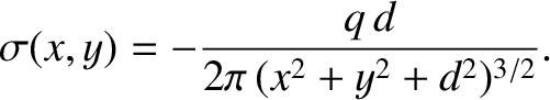
Figure 2.9:
The method of images for a charge and a grounded conducting plane.
|
|
Let us consider what do we know in this problem. We know that the conducting plate is an
equipotential surface. In fact, the potential of the plate is zero, because it is grounded.
We also know that the potential at infinity is zero (this is our usual boundary
condition for the scalar potential). Thus, we need to solve Poisson's equation, (2.99),
in the region  , with a single point charge located at coordinates (0, 0, ),
subject to the boundary conditions
, with a single point charge located at coordinates (0, 0, ),
subject to the boundary conditions
 |
(2.159) |
and
Let us forget about the real problem, for a
moment, and concentrate on a slightly different one. We shall refer to this as the
analog problem. See Figure 2.9. In the analog problem, we have a charge located at
coordinates (0, 0, ), and a charge  located at coordinates (0, 0, -), with no conductors present.
We can easily find the scalar potential for this problem, because we know where
all the charges are located. We get
located at coordinates (0, 0, -), with no conductors present.
We can easily find the scalar potential for this problem, because we know where
all the charges are located. We get
![$\displaystyle \phi_{\rm analog} (x, y, z) = \frac{1}{4\pi\,\epsilon_0}
\left[\frac{q}{\sqrt{x^2+y^2+(z-d)^2}}- \frac{q}{\sqrt{x^2+y^2+
(z+d)^2}}\right].$](img1420.png) |
(2.161) |
[See Equation (2.20).]
Note, however, that
 |
(2.162) |
and
Moreover, in the region ,
 satisfies Poisson's equation, (2.99),
for a point charge located at coordinates (0, 0, ). Thus, in this region,
is a solution
to the problem posed earlier. Now, the uniqueness theorem tells
us that there is only one solution to Poisson's equation
that satisfies a given well-posed set of boundary conditions. (See Section 2.1.10.) So,
must be the correct potential in the region .
Of course,
is completely wrong in the region
satisfies Poisson's equation, (2.99),
for a point charge located at coordinates (0, 0, ). Thus, in this region,
is a solution
to the problem posed earlier. Now, the uniqueness theorem tells
us that there is only one solution to Poisson's equation
that satisfies a given well-posed set of boundary conditions. (See Section 2.1.10.) So,
must be the correct potential in the region .
Of course,
is completely wrong in the region  .
We know this because the grounded plate shields the region from the
point charge, so that
.
We know this because the grounded plate shields the region from the
point charge, so that  in this region.
Now that we have found the potential in the region , we can easily work
out the distribution of charges induced on the conducting plate. We already
know that the relation between the electric
field immediately above a conducting surface
and the density of charge on the surface is
 |
(2.164) |
[See Equation (2.129).]
In this case,
 |
(2.165) |
so
 |
(2.166) |
It follows from Equation (2.161) that
![$\displaystyle \frac{\partial\phi_{\rm analog}}{\partial z} = \frac{q}{4\pi\,\ep...
...z-d)}{[x^2+y^2+(z-d)^2]^{3/2}} +
\frac{(z+d)}{[x^2+y^2+(z+d)^2]^{3/2}}\right\},$](img1429.png) |
(2.167) |
so
 |
(2.168) |
Clearly, the charge induced on the plate has the opposite sign to the point charge.
The charge density on the plate is also symmetric about the  -axis, and is largest
where the plate is closest to the point charge. The total charge induced on the
plate is
-axis, and is largest
where the plate is closest to the point charge. The total charge induced on the
plate is
 |
(2.169) |
which yields
 |
(2.170) |
where
 . Thus,
![$\displaystyle Q = - \frac{q\,d}{2} \int_0^\infty \frac{dk}{(k+d^2)^{3/2}}
= q\,d\left[ \frac{1}{(k+d^2)^{1/2}}\right]_0^\infty = - q.$](img1434.png) |
(2.171) |
So, the total charge induced on the plate is equal and opposite to the point charge that induces it.
As we have just seen, our point electric charge induces charges of the opposite sign on the conducting plate.
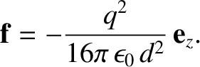
This, presumably, gives rise to a force of attraction between the charge and the
plate. What is this force? Well, because the potentials, and, hence, the electric
fields, in the vicinity of the point charge are the same in the real and analog problems,
the forces acting on this charge must be the same as well. In the analog problem,
there are two charges  a net distance
  apart. The force acting on
the charge at coordinates (0, 0, ) (i.e., the real charge) is
apart. The force acting on
the charge at coordinates (0, 0, ) (i.e., the real charge) is
 |
(2.172) |
[See Equation (2.2).]
Hence, this is also the force acting on the charge in the real problem.
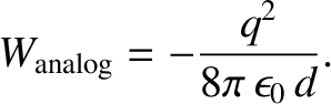
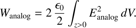
What, finally, is the potential energy of the system. For the analog problem
this is simply
 |
(2.173) |
[See Equation (2.69).]
Note that in the analog problem the fields on opposite sides of the conducting plate are mirror images
of one another, as are the charges (apart from the change
in sign). This is why the technique of replacing conducting surfaces by
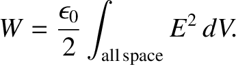
imaginary charges is called the method of images. We know that the potential
energy
of a set of charges is equivalent to the energy stored in the surrounding electric field.
Thus,
 |
(2.174) |
[See Equation (2.84).]
Moreover, as we just mentioned, in the analog problem, the fields on either side of the - plane are
mirror images of one another, so that
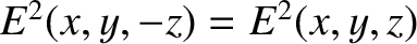 . It follows
that
. It follows
that
 |
(2.175) |
Now, in the real problem,
![\begin{displaymath}{\bf E} =\left\{
\begin{array}{lcl}
{\bf E}_{\rm analog}&\mbo...
...$z>0$}\\ [0.5ex]
{\bf0} &&\mbox{for $z <0$}
\end{array}\right..\end{displaymath}](img1441.png) |
(2.176) |
So,
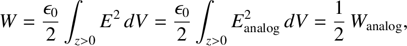 |
(2.177) |
giving
 |
(2.178) |
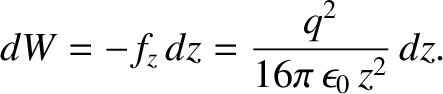
There is another method by which we can obtain the previous result. Suppose that
the point electric charge is gradually moved toward the plate along the -axis, starting from infinity,
until it reaches its final coordinates (0, 0, ). How much work is required to
achieve this? We know that the force of attraction acting on the charge is
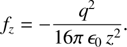 |
(2.179) |
[See Equation (2.172).]
Thus, the work required to move this charge by  is
is
 |
(2.180) |
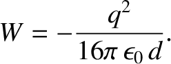
So, the total work needed to move the charge from  to
to  is
is
![$\displaystyle W = \frac{1}{4\pi\,\epsilon_0}\int_{\infty}^d \frac{q^2}{4\,z^2}\...
...t[ - \frac{q^2}{4 \,z} \right]_{\infty}^d
= - \frac{q^2}{16\pi\,\epsilon_0\,d}.$](img1448.png) |
(2.181) |
Of course, this work is equivalent to the potential energy (2.178),
and is, in turn, the same as the energy contained in the surrounding electric field.
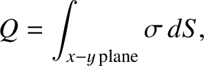
As a second example of the method of images, consider a grounded conducting sphere
of radius  centered on the origin. Suppose that a point electric charge is
placed outside the sphere at Cartesian coordinates
centered on the origin. Suppose that a point electric charge is
placed outside the sphere at Cartesian coordinates  , 0, 0), where
  . See Figure 2.10. What is
the force of attraction between the sphere and the charge? In this case,
we proceed by considering an analog problem in which the sphere is replaced by an image charge
. See Figure 2.10. What is
the force of attraction between the sphere and the charge? In this case,
we proceed by considering an analog problem in which the sphere is replaced by an image charge  placed
somewhere on the -axis at coordinates
placed
somewhere on the -axis at coordinates  , 0, 0). See Figure 2.10. The electric potential throughout space in the
analog problem is simply
, 0, 0). See Figure 2.10. The electric potential throughout space in the
analog problem is simply
![$\displaystyle \phi(x,y,z) = \frac{q}{4\pi\,\epsilon_0}\,\frac{1}{[(x-b)^2+y^2+z^2]^{1/2}}-\frac{q'}{4\pi\,\epsilon_0}
\frac{1}{[(x-c)^2+y^2+z^2]^{1/2}}.$](img1453.png) |
(2.182) |
[See Equation (2.20).]
Now, the image charge must be chosen so as to make the surface correspond to
the surface of the sphere. Setting the previous expression to zero, and performing
a little algebra, we find that the surface corresponds to
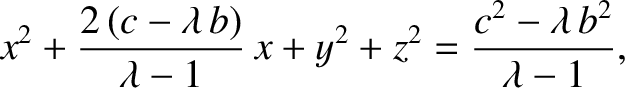 |
(2.183) |
where
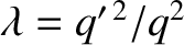 . Of course, the surface of the sphere satisfies
 |
(2.184) |
The previous two equations can be made identical by setting
 and
and
 ,
or
,
or
 |
(2.185) |
and
 |
(2.186) |
According to the uniqueness theorem, the potential in the analog problem is
now identical with that in the real problem in the region outside the sphere. (Of course, in the real
problem, the potential inside the sphere is zero.)
Hence, the
force of attraction between the sphere and the original charge in the real problem
is the same as the force of attraction between the image charge and the real charge in the analog
problem. It follows that
 |
(2.187) |
[See Equation (2.2).]
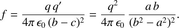
Figure 2.10:
The method of images for a charge and a grounded conducting sphere.
|
|
What is the total charge induced on the grounded conducting sphere? Well, according to
Gauss's law, the flux of the electric field out of a spherical Gaussian surface lying just
outside the surface of the conducting sphere is equal to the enclosed charge divided
by
 . (See Section 2.1.6.) In the real problem, the enclosed charge is the net
charge induced on the surface of the sphere. In the analog problem, the
enclosed charge is simply . However, the electric fields outside the
conducting sphere are identical in the real and analog problems. Hence, from Gauss's
law, the charge enclosed by the Gaussian surface must also be the same in both problems.
We thus conclude that the net charge induced on the surface of the conducting sphere is
. (See Section 2.1.6.) In the real problem, the enclosed charge is the net
charge induced on the surface of the sphere. In the analog problem, the
enclosed charge is simply . However, the electric fields outside the
conducting sphere are identical in the real and analog problems. Hence, from Gauss's
law, the charge enclosed by the Gaussian surface must also be the same in both problems.
We thus conclude that the net charge induced on the surface of the conducting sphere is
 |
(2.188) |
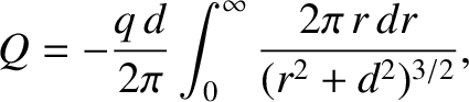
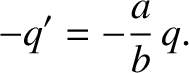
As another example of the method of images, consider an insulated, uncharged,
conducting sphere of radius , centered on the origin, in the presence of
a point electric charge placed outside the sphere at Cartesian coordinates  0, 0), where . See Figure 2.11. What is the force of attraction between the sphere
and the charge? Clearly, this new problem is very similar to the one that we just discussed. The only difference is that the surface of
the sphere is now at some unknown fixed potential
0, 0), where . See Figure 2.11. What is the force of attraction between the sphere
and the charge? Clearly, this new problem is very similar to the one that we just discussed. The only difference is that the surface of
the sphere is now at some unknown fixed potential  , and also carries zero net charge. Note that if we add a second image charge
  , located at the
origin, to the analog problem pictured in Figure 2.10 then the surface
, located at the
origin, to the analog problem pictured in Figure 2.10 then the surface  remains an equipotential surface. In fact, the potential of this surface becomes
 . [See Equation (2.20).] Moreover, the total charge enclosed
by the surface is
. [See Equation (2.20).] Moreover, the total charge enclosed
by the surface is  . This, of course, is the net charge induced on the
surface of the sphere in the real problem. Hence, we can see that if
. This, of course, is the net charge induced on the
surface of the sphere in the real problem. Hence, we can see that if
 then zero net charge is induced on the surface of the sphere. Thus, our
modified analog problem is now a solution to the problem under discussion, in the region outside the
sphere. See Figure 2.11. It follows that the surface of the sphere is at potential
then zero net charge is induced on the surface of the sphere. Thus, our
modified analog problem is now a solution to the problem under discussion, in the region outside the
sphere. See Figure 2.11. It follows that the surface of the sphere is at potential
 |
(2.189) |
Moreover, the force of attraction between the sphere and the original charge
in the real problem
is the same as the force of attraction between the image charges and the
real charge in the analog problem. Hence, the force is given by
 |
(2.190) |
[See Equation (2.2).]
Figure 2.11:
The method of images for a charge and an uncharged conducting sphere.
|
|
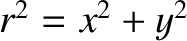
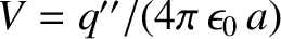
As a final example of the method of images, consider two identical, infinitely
long, conducting cylinders of radius that run parallel to the
-axis, and lie a distance apart. Suppose that one of the conductors
is held at potential  , while the other is held at potential
  . See Figure 2.12. What is the capacitance per unit length of the cylinders?
Consider an analog problem in which the conducting cylinders are replaced by
two infinitely long charge lines, of charge per unit length
 ,
that run parallel to the -axis, and lie a distance
,
that run parallel to the -axis, and lie a distance  apart. Now,
the potential in the - plane
generated by a charge line
apart. Now,
the potential in the - plane
generated by a charge line  running along the -axis
is
running along the -axis
is
 |
(2.191) |
where
 is the radial cylindrical polar coordinate. (See Section A.23.)
The corresponding electric field is radial, and satisfies
is the radial cylindrical polar coordinate. (See Section A.23.)
The corresponding electric field is radial, and satisfies
 |
(2.192) |
Incidentally, it is easily demonstrated from Gauss's law (see Section 2.1.6) that this is the correct electric field. Hence, the potential generated by two charge lines
located in the - plane at coordinates  , 0), respectively, is
Figure 2.12:
The method of images for two parallel cylindrical conductors.
|
|
Suppose that
 |
(2.194) |
where  is a constant.
It follows that
is a constant.
It follows that
 |
(2.195) |
Completing the square, we obtain
 |
(2.196) |
where
 |
(2.197) |
and
 |
(2.198) |
Of course, Equation (2.196) is the equation of a cylindrical surface of radius
centered on coordinates  , 0). Moreover, it follows from Equations (2.193) and (2.194) that this surface lies at the
constant potential
, 0). Moreover, it follows from Equations (2.193) and (2.194) that this surface lies at the
constant potential
 |
(2.199) |
Finally, it is easily demonstrated that the equipotential  corresponds
to a cylindrical surface of radius centered on
corresponds
to a cylindrical surface of radius centered on  . Hence, we can make
the analog problem match the real problem in the region outside
the cylinders by choosing
. Hence, we can make
the analog problem match the real problem in the region outside
the cylinders by choosing
 |
(2.200) |
Thus, we obtain
 |
(2.201) |
Now, it follows from Gauss's law (see Section 2.1.6), and the fact that the electric fields in the
real and analog problems are identical outside the cylinders, that the
charge per unit length stored on the surfaces of the two cylinders is
. Moreover,
the voltage difference between the cylinders is  . Hence, the
capacitance per unit length of the cylinders is
. Hence, the
capacitance per unit length of the cylinders is
 , yielding
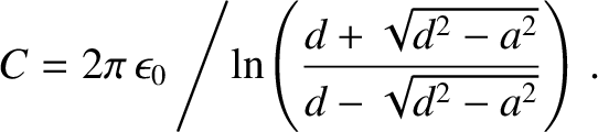 |
(2.202) |
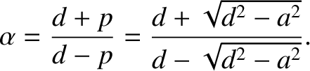
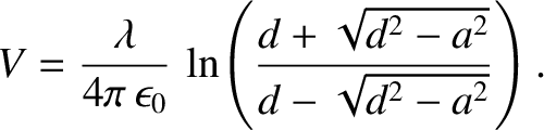
This expression simplifies to give
 |
(2.203) |
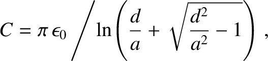
which can also be written
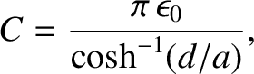 |
(2.204) |
because
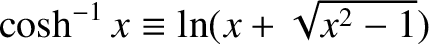 .
.

![\includegraphics[height=2.75in]{Chapter03/fig5_9.eps}](img1414.png)
![\includegraphics[height=2.5in]{Chapter03/fig5_10.eps}](img1462.png)
![\includegraphics[height=2.5in]{Chapter03/fig5_11.eps}](img1471.png)
![$\displaystyle =\frac{\lambda}{2\pi\,\epsilon_0}\,\ln\!\left[\frac{1}{\sqrt{(x-p...
...frac{\lambda}{2\pi\,\epsilon_0}\,\ln\!\left[\frac{1}{\sqrt{(x+p)^2+y^2}}\right]$](img1481.png)
![$\displaystyle = \frac{\lambda}{4\pi\,\epsilon_0}\,\ln\!\left[\frac{(x+p)^2+y^2}{(x-p)^2+y^2}\right].$](img1482.png)
![\includegraphics[height=2.25in]{Chapter03/fig5_12.eps}](img1483.png)