Next: Maxwell's Equations Up: Maxwell's Equations Previous: Maxwell's Equations
Prior to 1864, the laws of electromagnetism were written
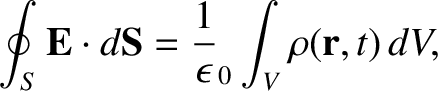
in integral form. Thus, Gauss's law (in SI units) was expressed as follows; the flux of
the electric field,
 , through a closed surface,
  , enclosing a volume,
  , is equal to the net enclosed electric charge,
divided by
, is equal to the net enclosed electric charge,
divided by
 ;
or
;
or
 |
(2.462) |
 is the electric charge density.
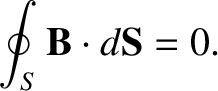
(See Section 2.1.6.) The no magnetic monopole law was expressed as follows; the flux of the
magnetic field,
is the electric charge density.
(See Section 2.1.6.) The no magnetic monopole law was expressed as follows; the flux of the
magnetic field,
 , through any closed surface, is zero;
or
, through any closed surface, is zero;
or
 |
(2.463) |
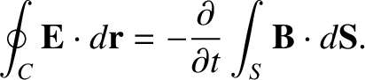
 , is equal to minus the
rate of change of the magnetic flux passing through any surface, , attached to the loop; or
, is equal to minus the
rate of change of the magnetic flux passing through any surface, , attached to the loop; or
 |
(2.464) |
is equal
the net current passing through any surface, , attached to the loop, multiplied by  ;
or
;
or
 |
(2.465) |
 is the electric current density. (See Section 2.2.10.)
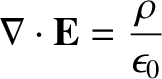
Maxwell's first great achievement was to realize that, with the aid of the divergence theorem and the curl theorem (see Sections A.20 and A.22), these laws could be re-expressed as a set of first-order partial differential equations. Of course, he wrote his equations out in component form, because modern vector notation did not come into vogue until about the time of the First World War. In modern notation, Maxwell first wrote:
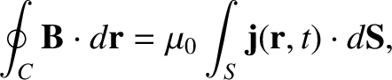
[See Equations (2.54), (2.263), (2.286), and (2.271).] Maxwell's second great achievement was to realize that these equations are not mathematically self-consistent.Consider the integral form of Equation (2.469):
This equation states that the line integral of the magnetic field around a closed loop is equal to the flux of the current density through the loop, multiplied by .
The problem is that the flux of the current density through a loop is not,
in general, a well-defined quantity.
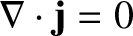
In order for the flux to be well defined, the integral of
 over some surface attached to a loop
must depend
on , but not on the details of . This is only the case if
over some surface attached to a loop
must depend
on , but not on the details of . This is only the case if
 |
(2.471) |
Why do we say that, in general,
 ? Consider
the flux of
? Consider
the flux of  out of some closed surface, , enclosing a
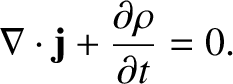
volume, . This is clearly equivalent to the instantaneous rate at which
electric charge flows out of . However, because electric charge is a conserved quantity (see Section 2.1.2), the rate at which charge flows out of must
equal
the rate of decrease of the charge contained in volume . Thus,
out of some closed surface, , enclosing a
volume, . This is clearly equivalent to the instantaneous rate at which
electric charge flows out of . However, because electric charge is a conserved quantity (see Section 2.1.2), the rate at which charge flows out of must
equal
the rate of decrease of the charge contained in volume . Thus,
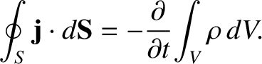 |
(2.472) |
 in a steady state situation; that is,
when
in a steady state situation; that is,
when
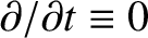 .
.
The problem with Ampère's circuital law is well illustrated by the following very famous
example.
Consider a long straight wire interrupted by a parallel plate capacitor. Suppose
that is some loop that circles the wire. In the time-independent case, the
capacitor acts like a break in the wire, so no current flows, and no magnetic
field is generated. There is clearly no problem with Ampère's circuital law in this case.
However, in the time-dependent case, a transient current flows in the wire as the
capacitor charges up, or charges down, and so a transient magnetic field is generated.
Thus, the line integral of the magnetic field around is
(transiently) non-zero. According to Ampère's circuital law, the flux of the current density
through any surface attached to should also be (transiently) non-zero.
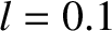
Let us consider two such surfaces. The
first surface,  , intersects the wire. See Figure 2.39. This surface
causes us no problem, because the flux of though the surface is clearly
non-zero (because the surface intersects
a current-carrying wire).
The second surface,
, intersects the wire. See Figure 2.39. This surface
causes us no problem, because the flux of though the surface is clearly
non-zero (because the surface intersects
a current-carrying wire).
The second surface,  , passes between the plates of the capacitor, and, therefore,
does not intersect the wire at all. Clearly, the flux of the current density through
this surface is zero. The current density fluxes through surfaces and
are obviously different. However, both surfaces are attached to the same loop ,
so
the fluxes should be the same, according to Ampère's circuital law, (2.470). Note, however, that although the surface does not intersect any electric current,
it does pass through a region containing a strong, time-varying
electric field, as it threads between the
plates of the charging (or discharging) capacitor. Perhaps, if we add a term involving
, passes between the plates of the capacitor, and, therefore,
does not intersect the wire at all. Clearly, the flux of the current density through
this surface is zero. The current density fluxes through surfaces and
are obviously different. However, both surfaces are attached to the same loop ,
so
the fluxes should be the same, according to Ampère's circuital law, (2.470). Note, however, that although the surface does not intersect any electric current,
it does pass through a region containing a strong, time-varying
electric field, as it threads between the
plates of the charging (or discharging) capacitor. Perhaps, if we add a term involving
 to the right-hand side of Equation (2.469) then we
can somehow fix up Ampère's circuital law? This is, essentially, how Maxwell reasoned
one hundred and fifty years ago.
to the right-hand side of Equation (2.469) then we
can somehow fix up Ampère's circuital law? This is, essentially, how Maxwell reasoned
one hundred and fifty years ago.
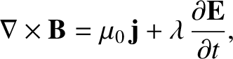
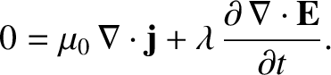
Let us try out this scheme. Suppose that we write
instead of Equation (2.469). Here, is some constant. Does this resolve
our problem? We require the flux of the right-hand side of the
previous equation through some loop to be well defined; that is, the flux should only
depend on , and not the particular surface (which spans ) upon which
it is evaluated. This is another way of saying that we require the divergence of
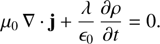
the right-hand side of the previous equation to be zero. (See Section A.20.) In fact, we can see that
this is necessary for mathematical self-consistency, because the divergence of the left-hand side
is identically zero. (See Section A.22.) So, taking the divergence of Equation (2.474), we obtain
is some constant. Does this resolve
our problem? We require the flux of the right-hand side of the
previous equation through some loop to be well defined; that is, the flux should only
depend on , and not the particular surface (which spans ) upon which
it is evaluated. This is another way of saying that we require the divergence of
the right-hand side of the previous equation to be zero. (See Section A.20.) In fact, we can see that
this is necessary for mathematical self-consistency, because the divergence of the left-hand side
is identically zero. (See Section A.22.) So, taking the divergence of Equation (2.474), we obtain
 |
(2.475) |
 |
(2.476) |
 |
(2.477) |
 |
(2.478) |
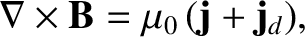
 . So, if we modify Equation (2.469)
such that it reads
where
. So, if we modify Equation (2.469)
such that it reads
where
 |
(2.480) |
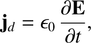
 ,
is known as the displacement current density (this name was invented by Maxwell).
In summary, we have shown that, although the flux of the real current density through a loop is
not well defined, if we form the sum of the real current density and the displacement
current density then the flux of this new quantity through a loop is well defined.
,
is known as the displacement current density (this name was invented by Maxwell).
In summary, we have shown that, although the flux of the real current density through a loop is
not well defined, if we form the sum of the real current density and the displacement
current density then the flux of this new quantity through a loop is well defined.
Of course, the displacement current is not a current at all. It is, in fact, associated with the induction of magnetic fields by time-varying electric fields. Maxwell came up with this rather curious name because many of his ideas regarding electric and magnetic fields were completely wrong. For instance, Maxwell believed in the aether (a tenuous invisible medium permeating all space; see Section 3.1.2), and he thought that electric and magnetic fields corresponded to stresses in this medium. He also thought that the displacement current was associated with a displacement of the aether (hence, the name). The reason that these misconceptions did not invalidate Maxwell's equations is quite simple. Maxwell based his equations on the results of experiments, and he added in his extra term so as to make these equations mathematically self-consistent. Both of these steps are valid irrespective of the existence or non-existence of the aether.
The field equations (2.466)–(2.469) are derived directly from the results of famous nineteenth century experiments. So, if a new term involving the time derivative of the electric field needs to be added to one of these equations, for the sake of mathematical consistency, why is there is no corresponding nineteenth century experimental result that demonstrates this fact? Actually, as is described in the following, the new term corresponds to an effect that is far too small to have been observed in the nineteenth century.
First, we shall show that it is comparatively easy to detect the induction of
an electric field by a changing magnetic field in a desktop laboratory experiment.
The Earth's magnetic field is about 1 gauss (that is,  tesla).
Magnetic fields generated by electromagnets (that will fit on a laboratory desktop)
are typically about one hundred times larger than this. Let us, therefore,
consider a hypothetical experiment in which a 100 gauss magnetic field is
switched on suddenly. Suppose that the field ramps up in one tenth of a second.
What electromotive force is generated in a 10 centimeter square loop of wire
located in this field? Faraday's law is written
tesla).
Magnetic fields generated by electromagnets (that will fit on a laboratory desktop)
are typically about one hundred times larger than this. Let us, therefore,
consider a hypothetical experiment in which a 100 gauss magnetic field is
switched on suddenly. Suppose that the field ramps up in one tenth of a second.
What electromotive force is generated in a 10 centimeter square loop of wire
located in this field? Faraday's law is written
 |
(2.481) |
 tesla is the magnetic field-strength,
  m
m the area of the loop,
and
the area of the loop,
and  seconds the ramp time. (See Section 2.3.1.) It follows that
 millivolt, which is easily detectable. In fact, most hand-held laboratory voltmeters
are calibrated in millivolts. It is, thus, clear that we would have no difficulty
whatsoever detecting the magnetic induction of electric fields in a nineteenth-century-style laboratory experiment.
millivolt, which is easily detectable. In fact, most hand-held laboratory voltmeters
are calibrated in millivolts. It is, thus, clear that we would have no difficulty
whatsoever detecting the magnetic induction of electric fields in a nineteenth-century-style laboratory experiment.
Let us now consider the electric induction of magnetic fields. Suppose that our
electric field is generated by a parallel plate capacitor of spacing one centimeter
that is charged up
to  volts. This gives an electric field of
  volts per meter. Suppose,
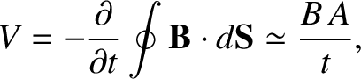
further, that the capacitor is discharged in one tenth of a second. The law
of electric induction is obtained by integrating Equation (2.479), and neglecting the
first term on the right-hand side. Thus,
volts per meter. Suppose,
further, that the capacitor is discharged in one tenth of a second. The law
of electric induction is obtained by integrating Equation (2.479), and neglecting the
first term on the right-hand side. Thus,
 |
(2.482) |
 |
(2.483) |
 meters is the dimensions of the loop,
  the
magnetic field-strength,
the
magnetic field-strength,
 volts per meter the electric field, and seconds the decay
time of the field. We obtain
volts per meter the electric field, and seconds the decay
time of the field. We obtain
 gauss. Modern technology is
unable to detect such
a small magnetic field, so we cannot really blame nineteenth century physicists for not
discovering electric induction experimentally.
gauss. Modern technology is
unable to detect such
a small magnetic field, so we cannot really blame nineteenth century physicists for not
discovering electric induction experimentally.
Note, however, that the displacement current is detectable in some modern experiments.
Suppose that we take an FM radio signal, amplify it so that its peak
voltage is one hundred volts, and then apply it to
the parallel plate capacitor in the previous hypothetical experiment.
What size of magnetic
field would this generate? A typical FM signal oscillates at  Hz,
so
Hz,
so  in the previous example changes from
  seconds to
  seconds.
Thus, the induced magnetic field is about
seconds.
Thus, the induced magnetic field is about  gauss. This
is certainly detectable by modern technology. Hence, we conclude that if the electric field is oscillating sufficiently rapidly then electric induction
of magnetic fields is an observable effect. In fact, there is a virtually
infallible rule for deciding whether or not the displacement current can be
neglected in Equation (2.479). Namely, if electromagnetic radiation is important
then the displacement current must be included. On the other hand, if
electromagnetic radiation is unimportant then the displacement current can be
safely neglected. Clearly, Maxwell's inclusion of the displacement current in
Equation (2.479) was a vital step in his later realization that his equations allowed
propagating wave-like solutions. These solutions
are, of course, electromagnetic waves.
gauss. This
is certainly detectable by modern technology. Hence, we conclude that if the electric field is oscillating sufficiently rapidly then electric induction
of magnetic fields is an observable effect. In fact, there is a virtually
infallible rule for deciding whether or not the displacement current can be
neglected in Equation (2.479). Namely, if electromagnetic radiation is important
then the displacement current must be included. On the other hand, if
electromagnetic radiation is unimportant then the displacement current can be
safely neglected. Clearly, Maxwell's inclusion of the displacement current in
Equation (2.479) was a vital step in his later realization that his equations allowed
propagating wave-like solutions. These solutions
are, of course, electromagnetic waves.


![\includegraphics[height=2in]{Chapter03/fig4_2.eps}](img2045.png)