Constant- Magnetic Island Evolution
Let us consider the nonlinear evolution of a chain of constant- magnetic islands whose thickness is
much greater than the linear layer thickness, but much less than the thickness of the equilibrium current sheet. In other words,
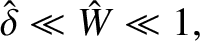 |
(9.88) |
where
 .
.
Writing
 ,
,
 ,
,
 ,
,
 , and
, and
 , the reduced-MHD equations, (9.11)–(9.14), become
in the limit
 ,
where
,
where
 |
(9.93) |
In the island region,
 ,
,  ,
,
 ,
,
 (this is
consistent with
(this is
consistent with
 ),
),
 (as will become apparent),
 (as will also become apparent), and
 . It follows that all terms in Equations (9.89) and (9.92) are of the same order of magnitude. On the other hand, the terms involving
  in Equation (9.90) are
smaller than the other term by a factor
in Equation (9.90) are
smaller than the other term by a factor
 . Finally, the term involving
  in Equation (9.91)
is smaller than the other terms by a factor
in Equation (9.91)
is smaller than the other terms by a factor  . Thus, to lowest order, Equations (9.89)–(9.92)
reduce to
. Thus, to lowest order, Equations (9.89)–(9.92)
reduce to
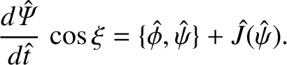
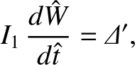
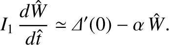
It is clear that the terms involving plasma inertia (i.e., the terms involving ) in the vorticity evolution equation
(9.90) become negligible as soon as the island width exceeds the linear layer width, leaving (9.95),
which corresponds to the force balance criterion
 . Thus, a nonlinear magnetic island
chain is essentially a
. Thus, a nonlinear magnetic island
chain is essentially a  -dependent magnetic equilibrium.
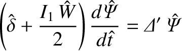
Equation (9.96) can be integrated to give
 |
(9.97) |
which is identical to the constant- result (9.83).
It follows that the constant- approximation is valid provided that
 . In other words,
provided that the perturbed current density in the island region is small compared to the equilibrium current
density.
. In other words,
provided that the perturbed current density in the island region is small compared to the equilibrium current
density.
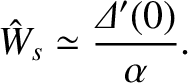
Equation (9.95) implies that
 |
(9.98) |
In other words, the current density in the island region is a flux-surface function (i.e., it is constant
on magnetic field-lines).
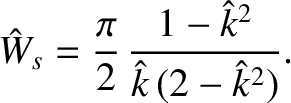
Equations (9.94), (9.97), and (9.98) can be combined to give
 |
(9.99) |
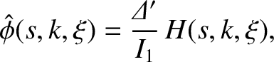
It is helpful to define
 . Writing
 , we find that
 |
(9.100) |
Thus, the contours of
 map out the magnetic field-lines in the vicinity of the
island chain. The region inside the magnetic separatrix corresponds to
map out the magnetic field-lines in the vicinity of the
island chain. The region inside the magnetic separatrix corresponds to
 , whereas the
region outside the separatrix corresponds to
, whereas the
region outside the separatrix corresponds to
 .
Let us transform into the new coordinate system
.
Let us transform into the new coordinate system
 ,
,
 , and
, and
 . It follows that
 . When written in terms of the new coordinates, the
plasma Ohm's law, (9.99), becomes
. When written in terms of the new coordinates, the
plasma Ohm's law, (9.99), becomes
 |
(9.101) |
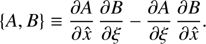
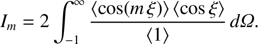
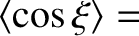
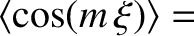
It is helpful to define the
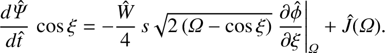
flux-surface average operator,
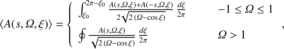 |
(9.102) |
where
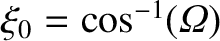 . The flux-surface average operator is designed to annihilate the
first term on the right-hand side of Equation (9.101). Thus, the flux-surface average of this
equation yields
. The flux-surface average operator is designed to annihilate the
first term on the right-hand side of Equation (9.101). Thus, the flux-surface average of this
equation yields
 |
(9.103) |
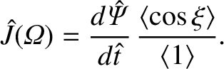
Let
 |
(9.104) |
which implies that
 . Equations (9.101) and (9.103) can
be combined to give
. Equations (9.101) and (9.103) can
be combined to give
 |
(9.105) |
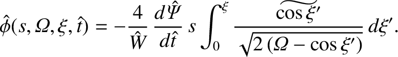
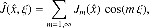
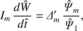
According to Equations (9.37), (9.91), and (9.102), asymptotic matching between the island solution and the
solution in the outer region (i.e., the region
 ) yields
Note that it is necessary to specifically project the  component out of
 because
is a nonlinear function that possesses many
because
is a nonlinear function that possesses many
 components, where
  ranges from
 to
to  . (See later.) Equations (9.103) and (9.106) can be combined to give
 |
(9.107) |
where
 |
(9.108) |
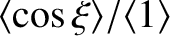
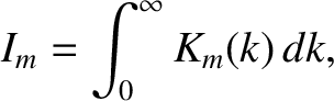
(See Table 9.1.) Equation (9.107) confirms that
(provided that
), as was previously assumed. Moreover, Equations (9.84), (9.103) and (9.107) demonstrate that the
constant- approximation (which requires
) is valid provided that
 |
(9.109) |
Note that this criterion becomes harder to satisfy as the island width grows, which implies that if the tearing mode is
in the constant- regime when it enters the nonlinear regime (i.e., if
 ) then it
may spontaneously leave the constant- regime as it subsequently evolves in time. (However, if
) then it
may spontaneously leave the constant- regime as it subsequently evolves in time. (However, if
 approaches unity when
then this indicates a
breakdown of asymptotic matching, due to the fact that the island width is no longer small compared to the
current sheet thickness, rather than a breakdown of the constant- approximation.) When written in unnormalized form,
the island width evolution equation, (9.107), yields the Rutherford island width evolution equation (Rutherford 1973),
approaches unity when
then this indicates a
breakdown of asymptotic matching, due to the fact that the island width is no longer small compared to the
current sheet thickness, rather than a breakdown of the constant- approximation.) When written in unnormalized form,
the island width evolution equation, (9.107), yields the Rutherford island width evolution equation (Rutherford 1973),
 |
(9.110) |
where
 is the island width in
  . According to the Rutherford equation, the growth of a constant-
tearing mode slows down as it enters the nonlinear regime (i.e., as the island width exceeds the
linear layer width). Indeed, the tearing mode transitions from growing exponentially in time on the
hybrid timescale
. According to the Rutherford equation, the growth of a constant-
tearing mode slows down as it enters the nonlinear regime (i.e., as the island width exceeds the
linear layer width). Indeed, the tearing mode transitions from growing exponentially in time on the
hybrid timescale
 to growing algebraically in time on the much
longer timescale
to growing algebraically in time on the much
longer timescale  .
.
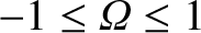
Figure: 9.6
Contours of the normalized perturbed current density distribution,
 ,
in the vicinity of a constant- magnetic island chain. Positive/negative
values are indicated by solid/dashed contours.
,
in the vicinity of a constant- magnetic island chain. Positive/negative
values are indicated by solid/dashed contours.
|
|
The current density in the island region that is specified in Equation (9.103) can be written in the form
 |
(9.111) |
where the
 are even functions of
  that are similar in magnitude to one another. (Note that there is no
  harmonic.) This is clear from
Figure 9.6, which shows contours of the normalized perturbed current density distribution,
. [See Equation (9.103).] It can be seen that the current density is mostly confined to the
interior of the magnetic separatrix, and becomes particularly large on the separatrix itself. (In fact,
the current density blows up logarithmically on the separatrix.) Clearly, such a current distribution cannot
be represented as
harmonic.) This is clear from
Figure 9.6, which shows contours of the normalized perturbed current density distribution,
. [See Equation (9.103).] It can be seen that the current density is mostly confined to the
interior of the magnetic separatrix, and becomes particularly large on the separatrix itself. (In fact,
the current density blows up logarithmically on the separatrix.) Clearly, such a current distribution cannot
be represented as
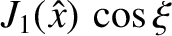 .
In other words, the current density distribution is multi-harmonic (i.e., it is not dominated by the
.
In other words, the current density distribution is multi-harmonic (i.e., it is not dominated by the  harmonic, but contains
substantial contributions from the
harmonic, but contains
substantial contributions from the  harmonics). It would seem reasonable, therefore, to write the solution to (9.96)
in the form
harmonics). It would seem reasonable, therefore, to write the solution to (9.96)
in the form
 |
(9.112) |
where the
 are independent of . However, when we actually wrote the solution to this equation, in
Equation (9.97), we omitted the higher harmonics (i.e., the
are independent of . However, when we actually wrote the solution to this equation, in
Equation (9.97), we omitted the higher harmonics (i.e., the
 for ). Let us now investigate under which circumstances this approximation can be justified. Let us, first of all, assume that the allowed wavenumbers
are quantized: that is,
for ). Let us now investigate under which circumstances this approximation can be justified. Let us, first of all, assume that the allowed wavenumbers
are quantized: that is,  , for
, for
 , where
 . (Here,
  is what we previously referred to
as
is what we previously referred to
as  .) Obviously, the easiest way to justify the quantization of the allowed wavenumbers is to
assume that the equilibrium current sheet has a finite length
.) Obviously, the easiest way to justify the quantization of the allowed wavenumbers is to
assume that the equilibrium current sheet has a finite length  in the -direction. Asymptotic matching between the island
solution and the solution in the outer region yields
in the -direction. Asymptotic matching between the island
solution and the solution in the outer region yields
 |
(9.113) |
where
 |
(9.114) |
Note that Equation (9.113) is the multi-harmonic generalization of Equation (9.107), Here,
 is what we previously referred to as
 , and
, and
 . Moreover,
 is the tearing stability index calculated with the
wavenumber
is the tearing stability index calculated with the
wavenumber  . (So
. (So
 is what we previously referred to as
 .)
Equation (9.113) yields
.)
Equation (9.113) yields
 |
(9.115) |
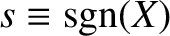
Figure: 9.7
Integrands for  integrals.
|
|
It is helpful to define
 . Thus,
  at the centers of the magnetic islands,
  on the magnetic separatrix, and
  in the region outside the separatrix.
It can be demonstrated that
in the region outside the separatrix.
It can be demonstrated that
where
are elliptic integrals (Abramowitz and Stegun 1965).
Hence, we can write
 |
(9.121) |
where
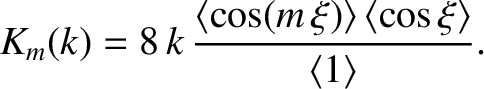 |
(9.122) |
Figure 9.7 shows the integands  . Note that all integrands are singular at the
magnetic separatrix (). However, the singularities are logarithmic in nature, and, therefore, integrable.
Note, further, that the higher order (i.e., ) integrands are of similar magnitude to the
integrand, which confirms that the
, for , appearing in Equation (9.111), are
of similar magnitude to
. Note that all integrands are singular at the
magnetic separatrix (). However, the singularities are logarithmic in nature, and, therefore, integrable.
Note, further, that the higher order (i.e., ) integrands are of similar magnitude to the
integrand, which confirms that the
, for , appearing in Equation (9.111), are
of similar magnitude to
 . In other words, the current density distribution is truly multi-harmonic.
However, it can be seen, from Figure 9.7, that the integrand is always positive, whereas the
integrands oscillate about zero. It is not surprising, therefore, that the
. In other words, the current density distribution is truly multi-harmonic.
However, it can be seen, from Figure 9.7, that the integrand is always positive, whereas the
integrands oscillate about zero. It is not surprising, therefore, that the  for
are much smaller in magnitude than
for
are much smaller in magnitude than  . In fact, as is shown in Table 9.1, the for
are, at least, 10 times smaller than . It follows from Equation (9.115)
that the single-harmonic approximation for
. In fact, as is shown in Table 9.1, the for
are, at least, 10 times smaller than . It follows from Equation (9.115)
that the single-harmonic approximation for
 (i.e., the neglect of the
for
) is justified as long as
(i.e., the neglect of the
for
) is justified as long as
 does not exceed the critical value
  , for .
As shown in Table 9.1, this is a comparatively easy criterion to meet, especially if the harmonic
is close to marginal stability (i.e.,
, for .
As shown in Table 9.1, this is a comparatively easy criterion to meet, especially if the harmonic
is close to marginal stability (i.e.,
 is small compared to unity).
Table: 9.1
The integrals for to  .
.
|
|
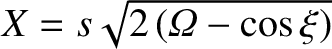
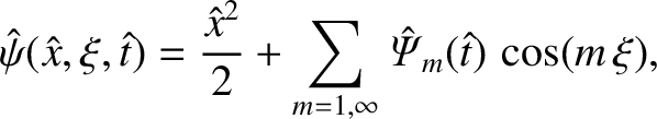
Figure: 9.8
Equally-spaced contours of the normalized stream-function,
 , in the vicinity of a constant-
magnetic island chain. Positive/negative
values are indicated by solid/dashed contours.
, in the vicinity of a constant-
magnetic island chain. Positive/negative
values are indicated by solid/dashed contours.
|
|
Equations (9.84), (9.105), and (9.107) yield
 |
(9.123) |
where
![\begin{displaymath}H(s,k,\xi)=s\left\{
\begin{array}{lll}
\frac{F(\varphi,k)\,E(...
...,1/k)\,E(\varphi',1/k)]}{F(\pi/2,1/k)}&&k>1
\end{array}\right.,\end{displaymath}](img3594.png) |
(9.124) |
and
Note that Equation (9.123) confirms that
in the island region (assuming that
), as was previously assumed. Figure 9.8 shows contours of the normalized stream-function,  , in the
- plane. It can be seen that the flow pattern associated with magnetic reconnection, which is clearly strongly multi-harmonic, is concentrated at the magnetic separatrix, being
particularly large at the magnetic X-points (Biskamp 1993). In fact, the flow velocity has a logarithmic singular on the magnetic
sepatratrix, indicating that plasma inertia cannot be neglected in the immediate vicinity of the sepatatrix. Consequently, an inertial layer [i.e., a layer in which plasma inertia cannot be neglected in Equation (9.90)], whose width is of order the linear layer width, develops on the separatrix. Fortunately,
the development of such a layer does not invalidate the results obtained in this section (Edery, et al., 1983). It is interesting to note that the
Rutherford island width evolution equation, (9.110), can be derived without explicitly calculating the flow pattern.
Nevertheless, the flow pattern is implicitly specified in the analysis.
, in the
- plane. It can be seen that the flow pattern associated with magnetic reconnection, which is clearly strongly multi-harmonic, is concentrated at the magnetic separatrix, being
particularly large at the magnetic X-points (Biskamp 1993). In fact, the flow velocity has a logarithmic singular on the magnetic
sepatratrix, indicating that plasma inertia cannot be neglected in the immediate vicinity of the sepatatrix. Consequently, an inertial layer [i.e., a layer in which plasma inertia cannot be neglected in Equation (9.90)], whose width is of order the linear layer width, develops on the separatrix. Fortunately,
the development of such a layer does not invalidate the results obtained in this section (Edery, et al., 1983). It is interesting to note that the
Rutherford island width evolution equation, (9.110), can be derived without explicitly calculating the flow pattern.
Nevertheless, the flow pattern is implicitly specified in the analysis.
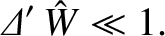
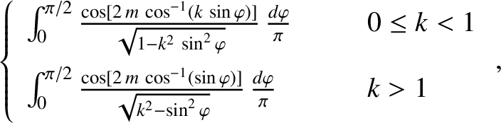
The island width evolution equation (9.107) seems to indicate that if
 then the island width, , grows without
limit. In fact, this is not the case. If we perform the asymptotic matching between the solution in the island
region and the solution in the outer region more carefully, taking the finite width of the magnetic island chain into account,
then the tearing stability index,
, which is defined in Equation (9.34), is replaced by (White, et al. 1977; Biskamp 1993)
then the island width, , grows without
limit. In fact, this is not the case. If we perform the asymptotic matching between the solution in the island
region and the solution in the outer region more carefully, taking the finite width of the magnetic island chain into account,
then the tearing stability index,
, which is defined in Equation (9.34), is replaced by (White, et al. 1977; Biskamp 1993)
![$\displaystyle {\mit\Delta}'(\hat{W}) =\frac{1}{\hat{\psi}(0)}\left[\frac{d\hat{\psi}(\bar{W}/2)}{d\hat{x}}- \frac{d\hat{\psi}(-\bar{W}/2)}{d\hat{x}}\right].$](img3599.png) |
(9.127) |
Here,
 is the average (over ) width of the magnetic separatrix, and
 is a solution of the tearing mode equation, (9.31). Making use of
Equation (9.36), we deduce that
is a solution of the tearing mode equation, (9.31). Making use of
Equation (9.36), we deduce that
 |
(9.128) |
where
 |
(9.129) |
for the specific plasma equilibrium discussed in Section 9.3. Here,
 is
specified in Equation (9.39). Thus, the modified island width evolution equation takes the form
is
specified in Equation (9.39). Thus, the modified island width evolution equation takes the form
 |
(9.130) |
It is clear from this equation that nonlinear growth of the tearing mode slows down, as the island width increases, and eventually stops when the island
width attains the value
 |
(9.131) |
For the specific equilibrium discussed in Section 9.3, the so-called saturated island width is
 |
(9.132) |
The previous expression is only accurate when
 (i.e., when the saturated island width
is much smaller than the width of the current sheet). This is only the case when
(i.e., when the saturated island width
is much smaller than the width of the current sheet). This is only the case when
 (i.e.,
when the tearing mode is close to marginal stability). However, it seems reasonable to deduce that if
then the tearing mode eventually attains a steady-state with a
saturated island
width that is comparable to the width of the equilibrium current sheet (i.e.,
(i.e.,
when the tearing mode is close to marginal stability). However, it seems reasonable to deduce that if
then the tearing mode eventually attains a steady-state with a
saturated island
width that is comparable to the width of the equilibrium current sheet (i.e.,
 ). In other words, the tearing mode completely
changes the topology of the current sheet's magnetic field on a timescale that is of order .
Equation (9.127) is only approximate. However, more rigorous calculations give essentially the
same result (Thyagararja, 1981; Escande & Ottaviani 2004; Militello & Porcelli 2004; Hastie, et al. 2005).
). In other words, the tearing mode completely
changes the topology of the current sheet's magnetic field on a timescale that is of order .
Equation (9.127) is only approximate. However, more rigorous calculations give essentially the
same result (Thyagararja, 1981; Escande & Ottaviani 2004; Militello & Porcelli 2004; Hastie, et al. 2005).
At first sight, the time evolution of a constant- tearing mode in the nonlinear regime seems completely
different to that in the linear regime. However, it turns out to be comparatively easy to formulate a theory that
takes both regimes into account. The time evolution of the tearing mode in the linear regime is specified by
 |
(9.133) |
Making use of Equation (9.60), this equation reduces to
 |
(9.134) |
where
![$\displaystyle \hat{\delta}=\left[\frac{2\pi\,\Gamma(3/4)}{\Gamma(1/4)}\right]^{4/5}{\mit\Delta}'^{1/5}\,S^{-2/5}$](img3612.png) |
(9.135) |
is the exact (normalized) linear layer width. The normalized Rutherford island width evolution equation, (9.107),
can be written
 |
(9.136) |
where use has been made of Equation (9.84). It can be seen, by comparison with Equation (9.134),
that a nonlinear magnetic island evolves in time in an analogous manner to a constant- linear layer
whose (normalized) thickness is
 . Thus, the essential nonlinearity in the nonlinear regime
arises because the effective layer width scales as the square root of the mode amplitude. [See Equation (9.84).] Recall that Equation (9.134) is valid when
. Thus, the essential nonlinearity in the nonlinear regime
arises because the effective layer width scales as the square root of the mode amplitude. [See Equation (9.84).] Recall that Equation (9.134) is valid when
 , whereas Equation (9.136) is valid when
 .
Thus, Equations (9.134)
and (9.136) can be combined to give the composite evolution equation
.
Thus, Equations (9.134)
and (9.136) can be combined to give the composite evolution equation
 |
(9.137) |
that interpolates between the linear and nonlinear regimes. As is clear, from the previous equation, the
magnetic reconnection rate decelerates in a smooth fashion as the island width exceeds the linear layer width.
Note, finally, that the type of slow magnetic reconnection, mediated by tearing modes that grow and eventually saturate, described in
this section is observed on a routine basis in tokamak plasmas (Wesson 2011).
![\includegraphics[height=3.8in]{Chapter09/fig9_6.eps}](img3537.png)

![\begin{align*}= \left\{
\begin{array}{lll}
K(\pi/2,k)/\pi&~~~~&0\leq k < 1\\ [2ex]
K(\pi/2,1/k)/k\,\pi&&k>1
\end{array}\right.,\end{align*}](img3565.png)
![\begin{align*}\left\{
\begin{array}{lll}
[K(\pi/2,k)-2\,E(\pi/2,k)]/\pi &~~~~&0\...
...\,K(\pi/2,1/k)-2\,k^2\,E(\pi/2,1/k)]/k\,\pi&&k>1
\end{array}\right.,\end{align*}](img3567.png)
![\includegraphics[height=3.8in]{Chapter09/fig9_8.eps}](img3591.png)

![$\displaystyle = \frac{\pi}{2}-{\rm sgn}(\xi)\,\cos^{-1}[\cos(\xi/2)/k],$](img3596.png)


![\includegraphics[height=3.75in]{Chapter09/fig9_7.eps}](img3559.png)