Next: Resistive Kink Modes Up: Magnetic Reconnection Previous: Asymptotic Matching Contents
 , and
, and
 .
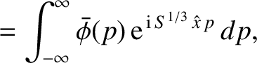
Equations (9.32) and (9.33) can be Fourier transformed, and the results combined, to
give
where
.
Equations (9.32) and (9.33) can be Fourier transformed, and the results combined, to
give
where
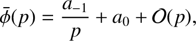
The most general small- asymptotic solution of Equation (9.45) is written
 and
and  are independent of , and it is assumed that
  .
When inverse Fourier transformed, the previous expression leads to the
following expression for the asymptotic behavior of
.
When inverse Fourier transformed, the previous expression leads to the
following expression for the asymptotic behavior of
 at the edge of
the layer (Erdéyli 1954):
at the edge of
the layer (Erdéyli 1954):
![$\displaystyle \skew{3}\hat{\phi}(\hat{x})= 2\,{\rm i}\left[\frac{a_0}{S^{1/3}\,\hat{x}} + \frac{\pi\,a_{-1}}{2}\,{\rm sgn}(\hat{x})
+{\cal O}(\hat{x}^2)\right].$](img3392.png) |
(9.48) |
 , is determined from the
small- asymptotic behavior of the Fourier-transformed layer solution.
, is determined from the
small- asymptotic behavior of the Fourier-transformed layer solution.
Let us search for an unstable perturbation characterized by  . It is
convenient to assume that
. It is
convenient to assume that
 approximation [because
it implies that
approximation [because
it implies that
 is approximately constant across the layer]
will be justified later on.
is approximately constant across the layer]
will be justified later on.
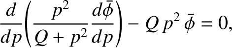
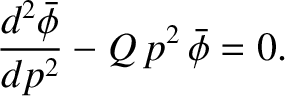
In the limit
 , Equation (9.45)
reduces to
, Equation (9.45)
reduces to
 is written
 , where
 is a standard parabolic cylinder function (Abramowitz and Stegun 1965). In the limit
we can make use of the standard small-argument expansion
of to write the most general solution to Equation (9.45) in the
form (Abramowitz and Stegun 1965)
Here,
is a standard parabolic cylinder function (Abramowitz and Stegun 1965). In the limit
we can make use of the standard small-argument expansion
of to write the most general solution to Equation (9.45) in the
form (Abramowitz and Stegun 1965)
Here,  is an arbitrary constant, and
  is a gamma function (Abramowitz and Stegun 1965).
In the limit
 |
(9.54) |
 |
(9.55) |
 and
and  are arbitrary constants.
Matching coefficients between Equations (9.53) and (9.56) in the range of
satisfying the inequality (9.52) yields the following expression
for the most general solution to Equation (9.45) in the limit
are arbitrary constants.
Matching coefficients between Equations (9.53) and (9.56) in the range of
satisfying the inequality (9.52) yields the following expression
for the most general solution to Equation (9.45) in the limit
 :
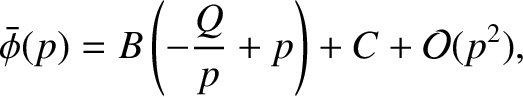
Finally, a comparison of Equations (9.47), (9.49), and (9.57)
gives the result
:
Finally, a comparison of Equations (9.47), (9.49), and (9.57)
gives the result
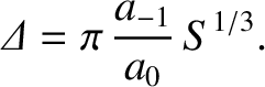
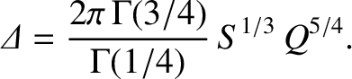
The asymptotic matching condition (9.42) can be combined with the previous
expression for
to give (Furth, Killeen, and Rosenbluth 1963)
 ,
,  , and
, and
 . According
to the previous equation, the perturbation, which is known as a tearing mode, is unstable whenever
. According
to the previous equation, the perturbation, which is known as a tearing mode, is unstable whenever
 , and grows on the hybrid timescale
 . [This hybrid growth time is consistent with our initial assumption (9.29), provided that
  .]
It is easily demonstrated that the tearing mode is stable whenever
.]
It is easily demonstrated that the tearing mode is stable whenever
 . Thus, we can now appreciate that
the solid curve in Figure 9.2, which is indented at the top (because
), is the outer solution of
an unstable tearing mode, whereas the dashed curve (which is not indented) is the outer solution of a stable
tearing mode.
Note, finally, that
. Thus, we can now appreciate that
the solid curve in Figure 9.2, which is indented at the top (because
), is the outer solution of
an unstable tearing mode, whereas the dashed curve (which is not indented) is the outer solution of a stable
tearing mode.
Note, finally, that
 as
as
 . In other words, the instability of the
current sheet when
is only made possible by finite plasma resistivity.
. In other words, the instability of the
current sheet when
is only made possible by finite plasma resistivity.
According to Equations (9.42), (9.50), and (9.58), the constant-
approximation holds provided that
 |
(9.61) |
Equation (9.51) implies that thickness of the layer in -space
is
 |
(9.62) |
 -space
is
When
-space
is
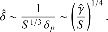
When
 then
then
 , according to
Equation (9.59), giving
, according to
Equation (9.59), giving
 . It is clear, therefore, that if
the Lundquist number, , is very large then the resistive layer centered
on the shear-Alfvén resonance,
. It is clear, therefore, that if
the Lundquist number, , is very large then the resistive layer centered
on the shear-Alfvén resonance,  , is extremely narrow compared to the width of the current sheet.
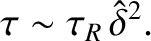
The timescale for magnetic flux to diffuse across a layer of thickness
 (in -space) is [see Equation (9.25)]
 |
(9.65) |
 , to be approximately
constant across the layer, because any non-uniformities in
would be
smoothed out via resistive diffusion. It follows from Equations (9.63) and (9.64)
that the constant- approximation holds provided that
, to be approximately
constant across the layer, because any non-uniformities in
would be
smoothed out via resistive diffusion. It follows from Equations (9.63) and (9.64)
that the constant- approximation holds provided that
 |
(9.66) |
 ), which is in agreement with Equation (9.50).


![$\displaystyle \skew{3}\bar{\phi}(p) = A\left[1- \frac{2\,\Gamma(3/4)}{\Gamma(1/4)}\, Q^{1/4}\,p + {\cal O}(p^{2})\right].$](img3403.png)
![$\displaystyle \skew{3}\bar{\phi} = A\,\left[\frac{2\,\Gamma(3/4)}{\Gamma(1/4)}\, \frac{Q^{5/4}}{p} + 1 + {\cal O}(p)\right].$](img3409.png)
![$\displaystyle \hat{\gamma} = \left[\frac{\Gamma(1/4)}{2\pi\,\Gamma(3/4)}\right]^{4/5}
{\mit\Delta}'^{\,4/5}\,S^{-3/5},$](img3411.png)
![$\displaystyle \gamma = \left[\frac{\Gamma(1/4)}{2\pi\,\Gamma(3/4)}\right]^{4/5}
\frac{{\mit\Delta}'^{\,4/5}}{\tau_H^{2/5}\,\tau_R^{3/5}}.$](img3412.png)