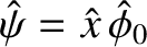
Next: Tearing Modes Up: Magnetic Reconnection Previous: Linearized Reduced-MHD Equations Contents
 , but much greater than
 . It follows that
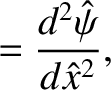
Thus, throughout much of the plasma, we can neglect the right-hand side of Equation (9.27), and the left-hand side of Equation (9.28), which is equivalent to the neglect of plasma resistivity and inertia. In this case,
Equations (9.27) and (9.28) reduce to
Equation (9.30) is simply the flux-freezing constraint that requires the plasma to move with the magnetic field.
Equation (9.31) is the linearized, static, force balance criterion:
. It follows that
Thus, throughout much of the plasma, we can neglect the right-hand side of Equation (9.27), and the left-hand side of Equation (9.28), which is equivalent to the neglect of plasma resistivity and inertia. In this case,
Equations (9.27) and (9.28) reduce to
Equation (9.30) is simply the flux-freezing constraint that requires the plasma to move with the magnetic field.
Equation (9.31) is the linearized, static, force balance criterion:
 .
Equations (9.30) and (9.31) are known collectively as the equations of marginally-stable ideal-MHD,
and are valid throughout virtually the whole plasma. However, it is clear that these equations break down in the
immediate vicinity of the shear-Alfvén resonance, where
.
Equations (9.30) and (9.31) are known collectively as the equations of marginally-stable ideal-MHD,
and are valid throughout virtually the whole plasma. However, it is clear that these equations break down in the
immediate vicinity of the shear-Alfvén resonance, where  (i.e., where the equilibrium magnetic field reverses direction). Observe, for instance, that the
  -component of the plasma velocity,
 , becomes infinite as
 ,
according to Equation (9.30).
,
according to Equation (9.30).
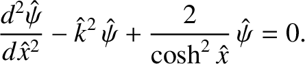
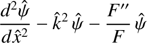
The marginally-stable ideal-MHD equations break down close to the shear-Alfvén resonance because the
neglect of plasma resistivity and inertia becomes untenable as
 . Thus, there is a thin
(compared to the current sheet thickness
. Thus, there is a thin
(compared to the current sheet thickness  ) layer,
centered on the resonance,
) layer,
centered on the resonance,  , where the behavior of the plasma is governed by the linearized reduced-MHD
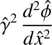
equations, (9.27) and (9.28). We can simplify these equations, making use of the
fact that
, where the behavior of the plasma is governed by the linearized reduced-MHD
equations, (9.27) and (9.28). We can simplify these equations, making use of the
fact that
 , and
, and
 , in a thin layer, to obtain the following layer equations:
 in the layer.
The stability problem reduces to solving the layer equations, (9.32) and (9.33), in the immediate vicinity of the shear-Alfvén resonance, , solving the marginally-stable ideal-MHD
equations, (9.30) and (9.31), everywhere else in the plasma, and matching the two solutions at the edge of the
layer. This method of solution,
which is known as asymptotic matching, was first described in a classic paper by Furth, Killeen, and
Rosenbluth (Furth, Killeen, and Rosenbluth 1963).
Let us consider the solution of the so-called tearing mode equation, (9.31), throughout the
bulk of the plasma. We could imagine launching a solution,
 , at large positive
  , which satisfies the physical boundary conditions as
 , and integrating this solution to the right-hand
boundary of the layer at
, and integrating this solution to the right-hand
boundary of the layer at
 . Likewise, we could also launch a
solution at large negative , which satisfies physical boundary conditions as
. Likewise, we could also launch a
solution at large negative , which satisfies physical boundary conditions as
 , and integrate this solution to the left-hand boundary of the layer at
 . Maxwell's
equations demand that
. Maxwell's
equations demand that
 be continuous on either side of the layer. Hence, we can multiply our two
solutions by appropriate factors, so as to ensure that
matches to the left and to the right of the layer.
This leaves the function
undetermined to an overall multiplicative constant, just as we would
expect in linear problem. In general,
be continuous on either side of the layer. Hence, we can multiply our two
solutions by appropriate factors, so as to ensure that
matches to the left and to the right of the layer.
This leaves the function
undetermined to an overall multiplicative constant, just as we would
expect in linear problem. In general,
 is not continuous to the left and to the
right of the layer. Thus, the marginally-stable ideal-MHD solution can be characterized by the
real number
is not continuous to the left and to the
right of the layer. Thus, the marginally-stable ideal-MHD solution can be characterized by the
real number
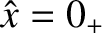
to the right and to the left of the layer. This
parameter is known as the tearing stability index, and is solely a property of the plasma equilibrium, the
wavenumber,  , and the boundary conditions imposed at infinity.
![\includegraphics[height=3.in]{Chapter09/fig9_2.eps}](img3351.png) |
Let us assume that the current sheet is isolated (i.e., it is not subject to any external magnetic perturbation). In this case,
the appropriate boundary conditions at
infinity are
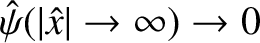 .
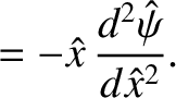
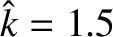
For the particular plasma equilibrium under consideration, for which
.
For the particular plasma equilibrium under consideration, for which
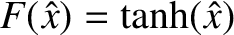 ,
the tearing mode equation, (9.31), takes the form
,
the tearing mode equation, (9.31), takes the form
 |
(9.35) |
 is an arbitrary constant. This solution is illustrated in Figure 9.2.
At the edge of the layer, which corresponds to the limit
is an arbitrary constant. This solution is illustrated in Figure 9.2.
At the edge of the layer, which corresponds to the limit
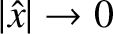 , the previous expression, in combination with Equation (9.30), yields
where
and use has been made of Equation (9.34).
As illustrated in Figure 9.3,
, the previous expression, in combination with Equation (9.30), yields
where
and use has been made of Equation (9.34).
As illustrated in Figure 9.3,
 for
for  ,
,
 for
for
 , and
, and
 as
as
 .
.
![\includegraphics[height=3.in]{Chapter09/fig9_3.eps}](img3369.png) |
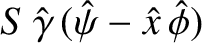
The layer equations, (9.32) and (9.33), possess the trivial twisting parity solution (Strauss, et al., 1979),
 ,
,
 , where
 is independent of . However, this solution cannot be matched to the so-called outer solution, (9.36), which has the opposite parity. Fortunately, the layer equations also possess a nontrivial tearing parity solution, such that
 and
and
 , which can be matched to the outer solution. The asymptotic
behavior of the tearing parity solution at the edge of the layer is
, which can be matched to the outer solution. The asymptotic
behavior of the tearing parity solution at the edge of the layer is
 is an arbitrary constant, and the parameter
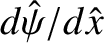
 is determined by solving the layer equations.
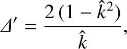
Matching Equations (9.37), (9.38), (9.40) and (9.41) at the edge of the layer yields
is determined by solving the layer equations.
Matching Equations (9.37), (9.38), (9.40) and (9.41) at the edge of the layer yields
 , and
The latter matching condition determines the growth-rate of the perturbation.
, and
The latter matching condition determines the growth-rate of the perturbation.


![$\displaystyle {\mit\Delta}' =\left[\frac{1}{\hat{\psi}}\,\frac{d\hat{\psi}}{d\hat{x}}\right]_{\hat{x}=0_-}^{\hat{x}=0_+}:$](img3350.png)

![$\displaystyle \rightarrow {\mit\Psi}\left[1 + \frac{{\mit\Delta}'}{2}\,\vert\hat{x}\vert +{\cal O}(\hat{x}^{\,2})\right],$](img3359.png)


![$\displaystyle \rightarrow{\mit\Psi}'\left[1+\frac{\mit\Delta}{2}\,\vert\hat{x}\vert+{\cal O}(\hat{x}^{\,2})\right],$](img3376.png)