Next: Plasmoid Instability Up: Magnetic Reconnection Previous: Constant- Magnetic Island Evolution Contents
![\includegraphics[height=3.8in]{Chapter09/fig9_9.eps}](img3618.png) |
We saw, in the last section, how a constant- tearing mode evolves in time after it enters the nonlinear regime.
Let us now consider how a non-constant- tearing mode evolves in time after it enters the nonlinear regime.
Recall, from Section 9.6, that a linear non-constant- tearing mode has a normalized layer thickness
tearing mode evolves in time after it enters the nonlinear regime.
Let us now consider how a non-constant- tearing mode evolves in time after it enters the nonlinear regime.
Recall, from Section 9.6, that a linear non-constant- tearing mode has a normalized layer thickness
 , a growth-rate
 , and is characterized by
 . Moreover, according to Section 9.7, the mode enters the nonlinear regime
as soon as
. Moreover, according to Section 9.7, the mode enters the nonlinear regime
as soon as
 exceeds
 , which implies that
 in the nonlinear regime. Hence, Equations (9.84) and (9.106) lead to the conclusion that
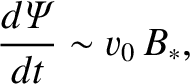
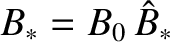
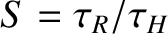
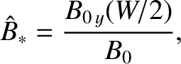
 in the nonlinear regime. In other words, the perturbed current density in the island region
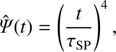
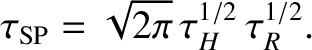
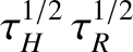
exceeds the equilibrium current density. Under these circumstances, both analytical calculations (Waelbroeck 1989) and numerical simulations (Biskamp 1993; Fitzpatrick 2003)
suggest that the solution to Equation (9.91) takes the form shown schematically in Figure 9.9.
It can be seen that the non-constant- magnetic islands only occupy the regions of the
in the nonlinear regime. In other words, the perturbed current density in the island region
exceeds the equilibrium current density. Under these circumstances, both analytical calculations (Waelbroeck 1989) and numerical simulations (Biskamp 1993; Fitzpatrick 2003)
suggest that the solution to Equation (9.91) takes the form shown schematically in Figure 9.9.
It can be seen that the non-constant- magnetic islands only occupy the regions of the  -axis in which
  , and are
connected by thin (compared to both the equilibrium current sheet thickness and the island width) current sheets that run along the resonant surface (
, and are
connected by thin (compared to both the equilibrium current sheet thickness and the island width) current sheets that run along the resonant surface ( ), and occupy the regions of the -axis in which
  .
.
Unfortunately, there is no known analytic solution of Equations (9.89)–(9.92) in the non-constant-
limit. However, we can still estimate the rate of magnetic reconnection using the
so-called the Sweet-Parker model (Sweet 1958; Parker 1957). The Sweet-Parker model concentrates on the dynamics of the current sheets that connect
the magnetic islands.
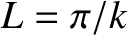
The
main features of the envisioned magnetic and plasma flow
fields in the vicinity of a given current sheet are illustrated in Figure 9.10. The reconnecting magnetic fields are anti-parallel,
and of equal strength,  .
The current sheet forms at the boundary between the
two fields, where the direction of the magnetic field suddenly changes,
and is assumed to be of thickness
.
The current sheet forms at the boundary between the
two fields, where the direction of the magnetic field suddenly changes,
and is assumed to be of thickness
 (in the
  -direction), and of length
  (in the
  -direction).
Plasma is assumed to diffuse into the current sheet, along its whole length,
at some relatively small inflow velocity,  . The plasma is accelerated
along the sheet, and eventually expelled from its two ends at some
relatively large exit velocity,
. The plasma is accelerated
along the sheet, and eventually expelled from its two ends at some
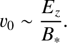
relatively large exit velocity,  . The inflow velocity
is simply an
. The inflow velocity
is simply an
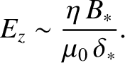
 velocity, so
 -component of Ohm's law yields
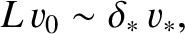
Continuity of plasma flow inside the sheet gives
assuming incompressible flow.
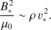
Pressure balance along the length of the sheet yields
Here, we have balanced the magnetic pressure at the center of the sheet
against the dynamic pressure of the outflowing plasma at the ends of the
sheet.
Finally, we can characterize the rate of reconnection via
the inflow velocity, , because all of the magnetic field-lines that are
convected into the sheet, along with the plasma, are eventually reconnected. In fact,
where
-component of Ohm's law yields
Continuity of plasma flow inside the sheet gives
assuming incompressible flow.
Pressure balance along the length of the sheet yields
Here, we have balanced the magnetic pressure at the center of the sheet
against the dynamic pressure of the outflowing plasma at the ends of the
sheet.
Finally, we can characterize the rate of reconnection via
the inflow velocity, , because all of the magnetic field-lines that are
convected into the sheet, along with the plasma, are eventually reconnected. In fact,
where
 is the (unnormalized) reconnected magnetic flux.
Let us adopt our standard normalizations:
 ,
,
 ,
,
 ,
,
 ,
,
 ,
,
 , where
  is specified in Equation (9.25). Equations (9.138) and (9.139) yield
 |
(9.143) |
 |
(9.144) |
 ,
,
 , and
, and  is specified in Equation (9.24). The previous equation
suggests that plasma is ejected from the ends of the current sheet at a velocity that is comparable with the
Alfvén velocity,
is specified in Equation (9.24). The previous equation
suggests that plasma is ejected from the ends of the current sheet at a velocity that is comparable with the
Alfvén velocity,
 . The length of a given Sweet-Parker current sheet is
 (recall that
 , where
  is a constant). Hence, the continuity equation (9.140)
implies that
is a constant). Hence, the continuity equation (9.140)
implies that
 |
(9.145) |
 |
 |
(9.146) |
 |
 |
(9.147) |
 times smaller than the equilibrium current sheet thickness. Finally,
the normalized version of Equation (9.142) yields
times smaller than the equilibrium current sheet thickness. Finally,
the normalized version of Equation (9.142) yields
Let us make the estimate
 |
(9.149) |
 , is specified in Equation (9.16), and
 is the full width of the magnetic island chain. [Here, we are assuming that (9.84) also applies to
non-constant- island chains.] Thus, in the small island width limit,
is the full width of the magnetic island chain. [Here, we are assuming that (9.84) also applies to
non-constant- island chains.] Thus, in the small island width limit,  , we get
Equations (9.148) and (9.150) can be combined to give
It follows that
assuming that
, we get
Equations (9.148) and (9.150) can be combined to give
It follows that
assuming that
 , where
 |
(9.153) |
tearing mode enters the nonlinear regime, complete magnetic reconnection
(i.e.,
 ) is achieved on the timescale
 . Note that this timescale is
considerably shorter than the timescale () needed for a nonlinear constant- tearing mode to
achieve full reconnection (because
. Note that this timescale is
considerably shorter than the timescale () needed for a nonlinear constant- tearing mode to
achieve full reconnection (because
 in a high Lundquist number plasma).
Equation (9.151) can also be written in the form
where is the non-constant- linear layer thickness. The previous equation confirms that the normalized Sweet-Parker
growth-rate matches the normalized non-constant- linear growth-rate (i.e.,
is the non-constant- linear layer thickness. The previous equation confirms that the normalized Sweet-Parker
growth-rate matches the normalized non-constant- linear growth-rate (i.e.,  ) at the boundary between the linear
and nonlinear regimes (i.e.,
) at the boundary between the linear
and nonlinear regimes (i.e.,
 ). Note that the reconnection rate decelerates slightly as the mode enters the nonlinear regime.
A nonlinear constant- tearing mode grows on the very long resistive timescale, , because plasma inertia
plays no role in the reconnection process. This is true despite the existence of an inertial layer on the magnetic
separatrix. (See Section 9.8.) On the other hand, a nonlinear non-constant- tearing mode grows on the much shorter hybrid timescale
 because plasma inertia is able to play a significant role
in the reconnection process within the Sweet-Parker current sheets that connect the magnetic islands (but remains negligible outside the sheets).
because plasma inertia is able to play a significant role
in the reconnection process within the Sweet-Parker current sheets that connect the magnetic islands (but remains negligible outside the sheets).
The Sweet-Parker reconnection ansatz is undoubtedly correct.
It has been simulated numerically many times, and was
confirmed experimentally in the Magnetic Reconnection Experiment (MRX)
operated by Princeton Plasma Physics Laboratory (PPPL) (Ji, et al. 1998). The problem is that
Sweet-Parker reconnection takes place far too slowly to account for
many reconnection processes that are thought to take place in the
solar system. For instance, in solar flares
 ,
,
 , and
, and
 (Priest 1984). According to the
Sweet-Parker model, magnetic energy is released to the plasma via
reconnection on a typical timescale of a few tens of days. In reality,
the energy is released in a few minutes to an hour (Priest 1984). Clearly, we can only hope to
account for solar flares using a reconnection mechanism that operates
far more rapidly than the Sweet-Parker mechanism.
(Priest 1984). According to the
Sweet-Parker model, magnetic energy is released to the plasma via
reconnection on a typical timescale of a few tens of days. In reality,
the energy is released in a few minutes to an hour (Priest 1984). Clearly, we can only hope to
account for solar flares using a reconnection mechanism that operates
far more rapidly than the Sweet-Parker mechanism.
![\includegraphics[height=2in]{Chapter09/fig9_10.eps}](img3629.png)