Three-Dimensional Wave Mechanics

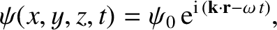
Up to now, we have only discussed wave mechanics for a particle moving in one dimension. However, the generalization to a particle moving in three dimensions is fairly straightforward. A massive particle moving in three dimensions has a complex wavefunction of the form [cf., Equation (4.10)]

$$\psi(x,y,z,t) = \psi_0\,{\rm e}^{{\rm i}\,({\bf k}\cdot{\bf r}-\omega\,t)},$$ (4.181)

where $\psi_0$ is a complex constant, and ${\bf r} = (x,\,y,\,z)$. Here, the wavevector, ${\bf k}$, and the angular frequency, $\omega$, are related to the particle momentum, ${\bf p}$, and energy, $E$, according to [cf., Equation (4.9)]

$${\bf p } = \hbar\,{\bf k},$$ (4.182)

and [cf., Equation (4.8)]

$$E =\hbar\,\omega,$$ (4.183)

respectively. Generalizing the analysis of Section 4.2.2, the three-dimensional version of Schrödinger's equation is [cf., Equation (4.22)]

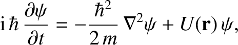$${\rm i}\,\hbar\,\frac{\partial\psi}{\partial t} = - \frac{\hbar^{2}}{2\,m}\,\nabla^{2}\psi + U({\bf r})\,\psi,$$ (4.184)

where the differential operator

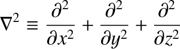$$\nabla^{2} \equiv \frac{\partial^{2}}{\partial x^{2}} + \frac{\partial^{2} }{\partial y^{2}} + \frac{\partial^{2}}{\partial z^{2}}$$ (4.185)

is known as the Laplacian. (See Section A.21.) The interpretation of a three-dimensional wavefunction is that the probability of simultaneously finding the particle between $x$ and $x+dx$, between $y$ and $y+dy$, and between $z$ and $z+dz$, at time $t$ is [cf., Equation (4.25)]

$$P(x,y,z,t) = \vert\psi(x,y,z,t)\vert^{2}\,dx\,dy\,dz.$$ (4.186)

Moreover, the normalization condition for the wavefunction becomes [cf., Equation (4.27)]

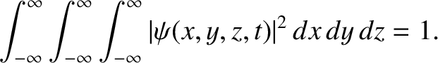$$\int_{-\infty}^\infty\int_{-\infty}^\infty\int_{-\infty}^\infty\vert\psi(x,y,z,t)\vert^{2}\,dx\,dy\,dz =1.$$ (4.187)

It can be demonstrated that Schrödinger's equation, (4.184), preserves the normalization condition, (4.187), of a localized wavefunction. Heisenberg's uncertainty principle generalizes to [cf., Equation (4.65)]

$${\mit\Delta} x\,{\mit\Delta} p_x\gtrsim \,\frac{\hbar}{2},$$ (4.188)

$${\mit\Delta} y\,{\mit\Delta} p_y\gtrsim \,\frac{\hbar}{2},$$ (4.189)

$${\mit\Delta} z\,{\mit\Delta} p_z\gtrsim \,\frac{\hbar}{2}.$$ (4.190)

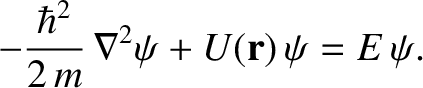
Finally, a stationary state of energy $E$ is written [cf., Equation (4.69)]

$$\psi(x,y,z,t) = \psi(x,y,z)\,{\rm e}^{-{\rm i}\,(E/\hbar)\,t},$$ (4.191)

where the stationary wavefunction, $\psi(x,y,z)$, satisfies [cf., Equation (4.71)]

$$- \frac{\hbar^{2}}{2\,m}\,\nabla^{2}\psi + U({\bf r})\,\psi = E\,\psi.$$ (4.192)